6 - Attention is All You Need
6 - Attention is All You Need
This part will be be implementing a (slightly modified version) of the Transformer model from the Attention is All You Need paper. For more information about the Transformer, see these three articles.
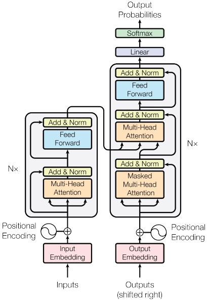
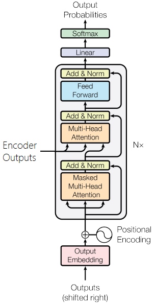
The left hand side is Encoder, the right hand side is Decoder. Full Architecture:
Introduction
The Transformer does not use any recurrence. It also does not use any convolutional layers. Instead the model is entirely made up of linear layers, attention mechanisms and normalization.
As of January 2020, Transformers are the dominant architecture in NLP and are used to achieve state-of-the-art results for many tasks and it appears as if they will be for the near future.
The most popular Transformer variant is BERT (Bidirectional Encoder Representations from Transformers) and pre-trained versions of BERT are commonly used to replace the embedding layers.
A common library used when dealing with pre-trained transformers is the Transformers library by huggingface, see here for a list of all pre-trained models available.
The differences between the implementation in this tutorial and the original paper are:
- Here use a learned positional encoding instead of a static one
- Here use the standard Adam optimizer with a static learning rate instead of one with warm-up and cool-down steps
- Here do not use label smoothing
- Here make all of these changes as they closely follow BERT’s set-up and the majority of Transformer variants use a similar set-up.
General Transformer Flow:
src -> Encoder -> Encoder Layers -> Self_attention(Multi-head attention) -> Positionwise_Feedforward -> Decoder -> Decoder Layers -> Self_attention(Multi-head attention) -> Self_attention(Multi-head attention) -> Encoder_decoder_attention(Multi-head attention) -> trg, attention
知识点:
- Encoder:
- Self-attention - 计算的是src或trg自身的词与词之间的依赖关系 (之前教程的Attention则是计算src的词与trg的词之间的依赖关系):
- 每个input token转成w2v
- 用w2v乘以三个权重矩阵(Wq,Wk,Wv)得到三个(Query,Key,Value)向量, q,k,v
- 用该位置token的q乘以自己以及其他token的k, 得到self-attention分数值
- 分数值除以一个常数(default 8), 让梯度更稳定, 然后放入softmax, 得到自己与其他每个token的权重
- 所有位置的权重乘以v并相加, 得到self-attention在该位置的输出,
$Z$ - 将上述总结成一个公式:
$A(Q,K,V) = softmax(\frac{QK^T}{\sqrt{d_k}})V = Z$
- Multi-Headed Attention - 扩展了模型专注于不同位置的能力:
- 把上述Self-attention的过程做8次, 即开始就初始化8组权重矩阵(Wq,Wk,Wv), 得到8个Q,K,V矩阵, 通过上述计算最后得到8个Z
- 将8个Z合并, 并乘以另一权重矩阵Wo, 最终得到一个Z矩阵
- Self-attention - 计算的是src或trg自身的词与词之间的依赖关系 (之前教程的Attention则是计算src的词与trg的词之间的依赖关系):
- Positional Encoding - 表示序列的顺序
- 将src的position放入到embedding layer
- Layer Normalization - 解决多层神经网络训练困难的问题,通过将前一层的信息无差的传递到下一层, 使特征的平均值为0, 标准差为1, 更容易训练
- Decoder
- 与 Encoder 相似, 但比Encoder多了一层Multi-Headed Attention
- 一层是src或trg自身的词与词之间的依赖关系, 另一层是是计算src的词与trg的词之间的依赖关系
- Mask
- Padding Mask - Encoder和Decoder都会用到, 大小与batch size对齐后序列一致,
的部分为0, 其余为1 - Sequence/Subsequent Mask - Decoder会用到, 为了使其看不到未来的信息(使Decoder输出应该只能依赖于 t 时刻之前的输出,而不能依赖 t 和 t 之后的输出), 通过下三角矩阵解决, 且下三角矩阵应与decoder的padding mask 结合
- Padding Mask - Encoder和Decoder都会用到, 大小与batch size对齐后序列一致,
Encoder:
- tokens are passed through a standard embedding layer
- token position in seqence are passed through a positional embedding layer
- token embeddings are multiplied by a scaling factor sqrt(d_model), d_model is the hidden dim size (reduces variance)
- token and positional embeddings are elementwise summed together to get a vector
- apply dropout to the combined embeddings
- combined embeddings are passed through encoder layer to get Z
- Encoder Layer:
- pass the source sentence and its mask into the multi-head attention layer
- apply dropout
- apply a residual connection and pass it through a Layer Normalization layer
- pass it through a position-wise feedforward
- apply dropout
- apply a residual connection and then layer normalization to get the output
Mutli Head Attention Layer:
- calculate Q,K,V with the linear layers
- split the hid_dim of the query, key and value into n_heads*head_dim
- multiply them together and then divide a scale (8=hid_dim//n_heads) to get the energy
- mask the energy
- apply the softmax to get attention
- apply dropout on attention and multiply with V to get x
- combine the n_head together
- multiply them with Wo
PositionwiseFeedforwardLayer:
- after attetnion operation, apply a fc layer first to transformed from hid_dim to pf_dim (512 to 2048)
- apply relu activation function (In BERT, use glue activation function)
- apply dropout
- apply another fc layer to transformed from pf_dim to hid_dim
Decoder:
- embedded target tokens, multiply a scale
- combines positional embeddings and scaled token embeddings - via an elementwise sum
- Apply dropout
- passed through the decoder layers
- passed through a linear layer
Decoder Layer:
- pass the target sentence and its mask into the multi-head attention layer (trg self one)
- apply dropout
- apply a residual connection and pass it through a Layer Normalization layer
- pass the target sentence,enc_src and src mask into the multi-head attention layer (src-trg one)
- apply dropout
- apply a residual connection and pass it through a Layer Normalization layer
- pass it through a position-wise feedforward
- apply dropout
- apply a residual connection and then layer normalization to get the output and attention
Seq2Seq:
Preparing Data
First, import all the required modules and set the random seeds for reproducability.
import torch
import torch.nn as nn
import torch.optim as optim

import torchtext
from torchtext.datasets import TranslationDataset, Multi30k
from torchtext.data import Field, BucketIterator

import matplotlib.pyplot as plt
import matplotlib.ticker as ticker

import spacy
import numpy as np

import random
import math
import time

SEED = 1234

random.seed(SEED)
np.random.seed(SEED)
torch.manual_seed(SEED)
torch.cuda.manual_seed(SEED)
torch.backends.cudnn.deterministic = True

spacy_de = spacy.load('de')
spacy_en = spacy.load('en')

# create tokenizer
def tokenize_de(text):
    """
    Tokenizes German text from a string into a list of strings
    """
    return [tok.text for tok in spacy_de.tokenizer(text)]

def tokenize_en(text):
    """
    Tokenizes English text from a string into a list of strings
    """
    return [tok.text for tok in spacy_en.tokenizer(text)]
The model expects data to be fed in with the batch dimension first, so here use batch_first = True.
SRC = Field(tokenize=tokenize_de,
            init_token = '<sos>',
            eos_token = '<eos>',
            lower = True,
            batch_first = True)

TRG = Field(tokenize = tokenize_en,
            init_token = '<sos>',
            eos_token = '<eos>',
            lower = True,
            batch_first = True)

# Load data
train_data, valid_data, test_data = Multi30k.splits(exts = ('.de', '.en'), fields = (SRC, TRG))
print(vars(train_data.examples[0]))
# {'src': ['zwei', 'junge', 'weiße', 'männer', 'sind', 'im', 'freien', 'in', 'der', 'nähe', 'vieler', 'büsche', '.'], 'trg': ['two', 'young', ',', 'white', 'males', 'are', 'outside', 'near', 'many', 'bushes', '.']}

# Build the vocabulary
SRC.build_vocab(train_data, min_freq = 2)
TRG.build_vocab(train_data, min_freq = 2)
The final bit of data preparation is defining the device and then building the iterator.
device = torch.device('cuda' if torch.cuda.is_available() else 'cpu')

BATCH_SIZE = 128

train_iterator, valid_iterator, test_iterator = BucketIterator.splits(
    (train_data, valid_data, test_data),
     batch_size = BATCH_SIZE,
     device = device)
Building the Seq2Seq Model
Encoder
The Transformer’s encoder does not attempt to compress the entire source sentence, $X = (x_1, ... ,x_n)$, into a single context vector, $z$. Instead it produces a sequence of context vectors, $Z = (z_1, ... , z_n)$. So, if input sequence was 5 tokens long, it would have $Z = (z_1, z_2, z_3, z_4, z_5)$. It is called a sequence of context vectors instead of a sequence of hidden states, because A hidden state at time $t$ in an RNN has only seen tokens $x_t$ and all the tokens before it. However, each context vector here has seen all tokens at all positions within the input sequence.
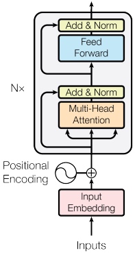
First, the tokens are passed through a standard embedding layer. Next, as the model has no recurrent it has no idea about the order of the tokens within the sequence. It can be solved by using a second embedding layer called a positional embedding layer. This is a standard embedding layer where the input is the position of the token within the sequence, starting with the first token, the
The original Transformer implementation from the Attention is All You Need paper does not learn positional embeddings. Instead it uses a fixed static embedding. Modern Transformer architectures, like BERT, use positional embeddings instead, hence here use them in these tutorials. Check out this section to read more about the positional embeddings used in the original Transformer model.
Next, the token and positional embeddings are elementwise summed together to get a vector which contains information about the token and also its position with in the sequence. However, before they are summed, the token embeddings are multiplied by a scaling factor which is $\sqrt{d_{model}}$, where $d_{model}$ is the hidden dimension size, hid_dim. This supposedly reduces variance in the embeddings and the model is difficult to train reliably without this scaling factor. Dropout is then applied to the combined embeddings.
The combined embeddings are then passed through $N$ encoder layers to get $Z$, which is then output and can be used by the decoder.
The source mask, src_mask, is simply the same shape as the source sentence but has a value of 1 when the token in the source sentence is not a
class Encoder(nn.Module):
    def __init__(self,
                 input_dim,
                 hid_dim,
                 n_layers,
                 n_heads,
                 pf_dim,
                 dropout,
                 device,
                 max_length = 100):
        super().__init__()

        self.device = device

        self.tok_embedding = nn.Embedding(input_dim, hid_dim)
        self.pos_embedding = nn.Embedding(max_length, hid_dim)

        self.layers = nn.ModuleList([EncoderLayer(hid_dim,
                                                  n_heads,
                                                  pf_dim,
                                                  dropout,
                                                  device)
                                     for _ in range(n_layers)])

        self.dropout = nn.Dropout(dropout)

        self.scale = torch.sqrt(torch.FloatTensor([hid_dim])).to(device)

    def forward(self, src, src_mask):

        #src = [batch size, src len]
        #src_mask = [batch size, src len]

        batch_size = src.shape[0]
        src_len = src.shape[1]

        pos = torch.arange(0, src_len).unsqueeze(0).repeat(batch_size, 1).to(self.device)

        #pos = [batch size, src len]

        src = self.dropout((self.tok_embedding(src) * self.scale) + self.pos_embedding(pos))

        #src = [batch size, src len, hid dim]

        for layer in self.layers:
            src = layer(src, src_mask)

        #src = [batch size, src len, hid dim]

        return src
Encoder Layer
First, pass the source sentence and its mask into the multi-head attention layer, then perform dropout on it, apply a residual connection and pass it through a Layer Normalization layer. Then pass it through a position-wise feedforward layer and then, again, apply dropout, a residual connection and then layer normalization to get the output of this layer which is fed into the next layer. The parameters are not shared between layers.
The mutli head attention layer is used by the encoder layer to attend to the source sentence, i.e. it is calculating and applying attention over itself instead of another sequence, hence call it self attention.
This article goes into more detail about layer normalization, but the gist is that it normalizes the values of the features, i.e. across the hidden dimension, so each feature has a mean of 0 and a standard deviation of 1. This allows neural networks with a larger number of layers, like the Transformer, to be trained easier.
class EncoderLayer(nn.Module):
    def __init__(self,
                 hid_dim,
                 n_heads,
                 pf_dim,
                 dropout,
                 device):
        super().__init__()

        self.self_attn_layer_norm = nn.LayerNorm(hid_dim)
        self.ff_layer_norm = nn.LayerNorm(hid_dim)
        self.self_attention = MultiHeadAttentionLayer(hid_dim, n_heads, dropout, device)
        self.positionwise_feedforward = PositionwiseFeedforwardLayer(hid_dim,
                                                                     pf_dim,
                                                                     dropout)
        self.dropout = nn.Dropout(dropout)

    def forward(self, src, src_mask):

        #src = [batch size, src len, hid dim]
        #src_mask = [batch size, src len]

        #self attention
        _src, _ = self.self_attention(src, src, src, src_mask) # multi-head( query, key, value, mask = None)

        #dropout, residual connection and layer norm
        src = self.self_attn_layer_norm(src + self.dropout(_src))

        #src = [batch size, src len, hid dim]

        #positionwise feedforward
        _src = self.positionwise_feedforward(src)

        #dropout, residual and layer norm
        src = self.ff_layer_norm(src + self.dropout(_src))

        #src = [batch size, src len, hid dim]

        return src
Mutli Head Attention Layer
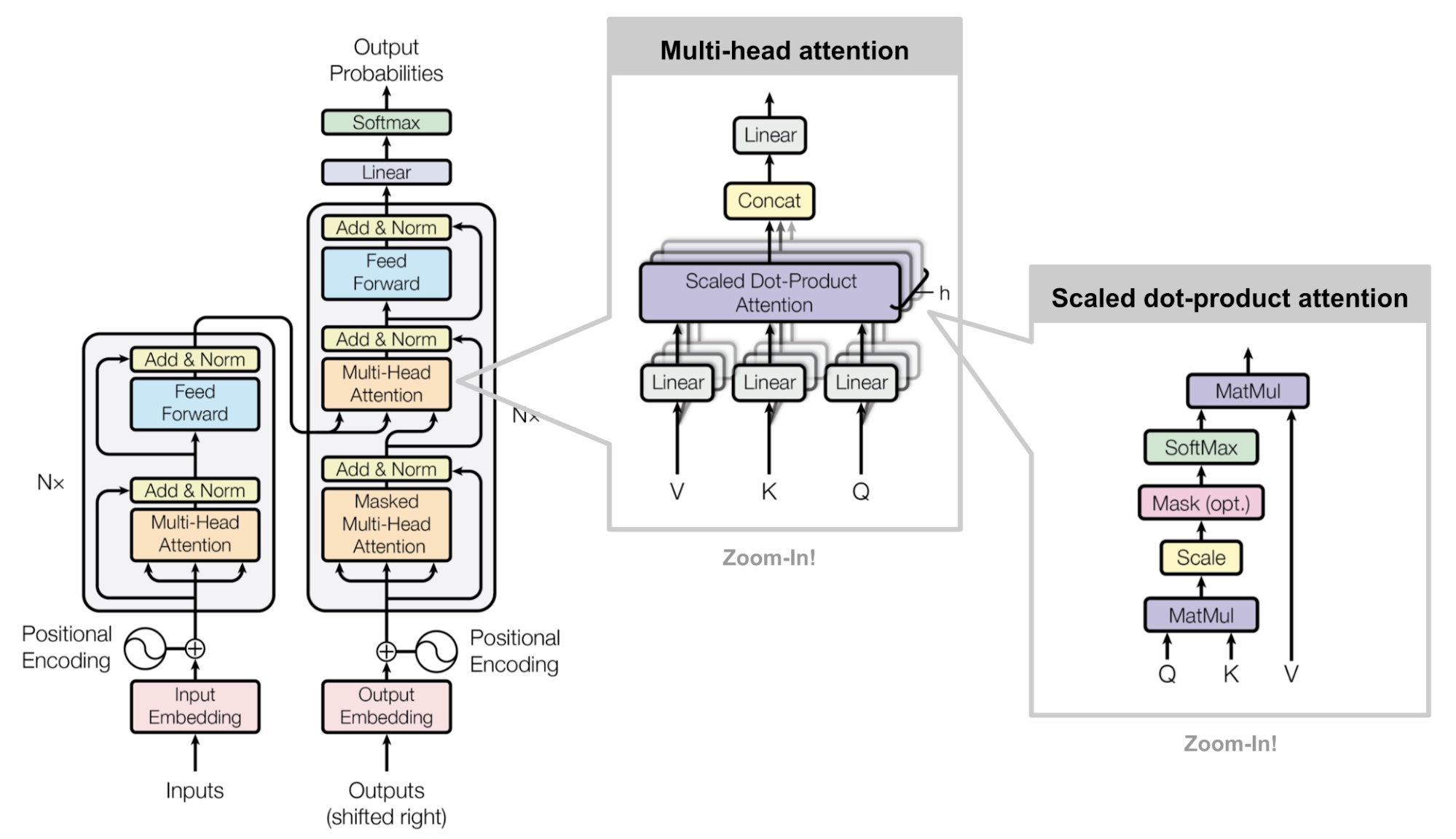
One of the key, novel concepts introduced by the Transformer paper is the multi-head attention layer.
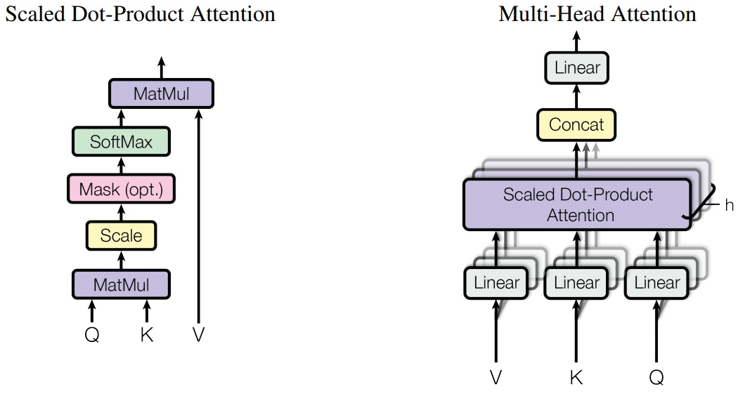
Attention can be though of as queries, keys and values - where the query is used with the key to get an attention vector (usually the output of a softmax operation and has all values between 0 and 1 which sum to 1) which is then used to get a weighted sum of the values.
The Transformer uses scaled dot-product attention, where the query and key are combined by taking the dot product between them, then applying the softmax operation and scaling by $d_k$ before finally then multiplying by the value. $d_k$ is the head dimension, head_dim.
$$ \text{Attention}(Q, K, V) = \text{Softmax} \big( \frac{QK^T}{\sqrt{d_k}} \big)V $$
This is similar to standard dot product attention but is scaled by $d_k$, which the paper states is used to stop the results of the dot products growing large, causing gradients to become too small.
However, the scaled dot-product attention isn’t simply applied to the queries, keys and values. Instead of doing a single attention application the queries, keys and values have their hid_dim split into $h$ heads and the scaled dot-product attention is calculated over all heads in parallel. This means instead of paying attention to one concept per attention application, it pay attention to $h$. Then re-combine the heads into their hid_dim shape, thus each hid_dim is potentially paying attention to $h$ different concepts.
$$ \text{MultiHead}(Q, K, V) = \text{Concat}(\text{head}_1,...,\text{head}_h)W^O $$
$$\text{head}_i = \text{Attention}(QW_i^Q, KW_i^K, VW_i^V) $$
$W^O$ is the linear layer applied at the end of the multi-head attention layer, fc. $W^Q, W^K, W^V$ are the linear layers fc_q, fc_k and fc_v.
Walking through the module, first calculate $QW^Q$, $KW^K$ and $VW^V$ with the linear layers, fc_q, fc_k and fc_v, to give Q, K and V. Next, split the hid_dim of the query, key and value into n_heads (hid_dim=n_heads*head_dim) using .view and correctly permute them so they can be multiplied together. Then calculate the energy (the un-normalized attention) by multiplying Q and K together and scaling it by the square root of head_dim, which is calulated as hid_dim // n_heads. Then mask the energy so it does not pay attention over any elements of the sequeuence, then apply the softmax and dropout. Then apply the attention to the value heads, V, before combining the n_heads together. Finally, multiply this $W^O$, represented by fc_o.
Note that in implementation the lengths of the keys and values are always the same, thus when matrix multiplying the output of the softmax, attention, with V we will always have valid dimension sizes for matrix multiplication. This multiplication is carried out using torch.matmul which, when both tensors are >2-dimensional, does a batched matrix multiplication over the last two dimensions of each tensor. This will be a [query len, key len] x [value len, head dim] batched matrix multiplication over the batch size and each head which provides the [batch size, n heads, query len, head dim] result.
One thing that looks strange at first is that dropout is applied directly to the attention. This means that attention vector will most probably not sum to 1 and may pay full attention to a token but the attention over that token is set to 0 by dropout. This is never explained, or even mentioned, in the paper however is used by the official implementation and every Transformer implementation, including BERT.
class MultiHeadAttentionLayer(nn.Module):
    def __init__(self, hid_dim, n_heads, dropout, device):
        super().__init__()

        assert hid_dim % n_heads == 0

        self.hid_dim = hid_dim   # in paper, 512
        self.n_heads = n_heads   # in paper, 8
        self.head_dim = hid_dim // n_heads  # in paper, 512 // 8 = 64

        self.fc_q = nn.Linear(hid_dim, hid_dim)
        self.fc_k = nn.Linear(hid_dim, hid_dim)
        self.fc_v = nn.Linear(hid_dim, hid_dim)

        self.fc_o = nn.Linear(hid_dim, hid_dim)

        self.dropout = nn.Dropout(dropout)

        self.scale = torch.sqrt(torch.FloatTensor([self.head_dim])).to(device)  # sqrt(64)

    def forward(self, query, key, value, mask = None):

        batch_size = query.shape[0]

        #query = [batch size, query len, hid dim]
        #key = [batch size, key len, hid dim]
        #value = [batch size, value len, hid dim]

        Q = self.fc_q(query)
        K = self.fc_k(key)
        V = self.fc_v(value)

        #Q = [batch size, query len, hid dim]
        #K = [batch size, key len, hid dim]
        #V = [batch size, value len, hid dim]

        Q = Q.view(batch_size, -1, self.n_heads, self.head_dim).permute(0, 2, 1, 3)
        K = K.view(batch_size, -1, self.n_heads, self.head_dim).permute(0, 2, 1, 3)
        V = V.view(batch_size, -1, self.n_heads, self.head_dim).permute(0, 2, 1, 3)

        #Q = [batch size, n heads, query len, head dim]
        #K = [batch size, n heads, key len, head dim]
        #V = [batch size, n heads, value len, head dim]

        energy = torch.matmul(Q, K.permute(0, 1, 3, 2)) / self.scale

        #energy = [batch size, n heads, query len, key len]

        if mask is not None:
            energy = energy.masked_fill(mask == 0, -1e10)

        attention = torch.softmax(energy, dim = -1)

        #attention = [batch size, n heads, query len, key len]

        x = torch.matmul(self.dropout(attention), V)  #x = [batch size, n heads, query len, head dim]

        # 将x还原成linear layer可以process的size
        x = x.permute(0, 2, 1, 3).contiguous()
        # contiguous 返回一个内存连续的有相同数据的tensor,如果原tensor内存连续,则返回原tensor. 一般与transpose,permute, view搭配使用
        # transpose、permute等维度变换操作后,tensor在内存中不再是连续存储的,而view操作要求tensor的内存连续存储,所以需要contiguous来返回一个contiguous copy


        x = x.view(batch_size, -1, self.hid_dim) #x = [batch size, query len, n heads, head dim]

        x = self.fc_o(x) #x = [batch size, query len, hid dim]

        return x, attention
Position-wise Feedforward Layer
The other main block inside the encoder layer is the position-wise feedforward layer. The input is transformed from hid_dim to pf_dim, where pf_dim is usually a lot larger than hid_dim. The original Transformer used a hid_dim of 512 and a pf_dim of 2048. The ReLU activation function and dropout are applied before it is transformed back into a hid_dim representation.
Why is this used? Unfortunately, it is never explained in the paper.
BERT uses the GELU activation function, which can be used by simply switching torch.relu for F.gelu. Why did they use GELU? Again, it is never explained.
class PositionwiseFeedforwardLayer(nn.Module):
    def __init__(self, hid_dim, pf_dim, dropout):
        super().__init__()

        self.fc_1 = nn.Linear(hid_dim, pf_dim)
        self.fc_2 = nn.Linear(pf_dim, hid_dim)

        self.dropout = nn.Dropout(dropout)

    def forward(self, x):

        #x = [batch size, seq len, hid dim]

        x = self.dropout(torch.relu(self.fc_1(x)))

        #x = [batch size, seq len, pf dim]

        x = self.fc_2(x)

        #x = [batch size, seq len, hid dim]

        return x
Decoder
The objective of the decoder is to take the encoded representation of the source sentence, $Z$, and convert it into predicted tokens in the target sentence, $\hat{Y}$. Then compare $\hat{Y}$ with the actual tokens in the target sentence, $Y$, to calculate loss, which will be used to calculate the gradients of parameters and then use optimizer to update weights in order to improve predictions.
The decoder is similar to encoder, however it now has two multi-head attention layers. A masked multi-head attention layer over the target sequence, and a multi-head attention layer which uses the decoder representation as the query and the encoder representation as the key and value. (两个multi-head attention layer, 一个为计算trg自身的词之间的attention, 一个是计算src与trg词之间的attention)
The decoder uses positional embeddings and combines - via an elementwise sum - them with the scaled embedded target tokens, followed by dropout. Again, positional encodings have a “vocabulary” of 100, which means they can accept sequences up to 100 tokens long. This can be increased if desired.
The combined embeddings are then passed through the $N$ decoder layers, along with the encoded source, enc_src, and the source and target masks. Note that the number of layers in the encoder does not have to be equal to the number of layers in the decoder, even though they are both denoted by $N$.
The decoder representation after the $N^{th}$ layer is then passed through a linear layer, fc_out. In PyTorch, the softmax operation is contained within loss function, so do not explicitly need to use a softmax layer here.
As well as using the source mask to prevent model attending to
Decoder layer also outputs the normalized attention values so can later plot them to see what model is actually paying attention to.
    def __init__(self,
                 output_dim,
                 hid_dim,
                 n_layers,
                 n_heads,
                 pf_dim,
                 dropout,
                 device,
                 max_length = 100):
        super().__init__()

        self.device = device

        self.tok_embedding = nn.Embedding(output_dim, hid_dim)
        self.pos_embedding = nn.Embedding(max_length, hid_dim)

        self.layers = nn.ModuleList([DecoderLayer(hid_dim,
                                                  n_heads,
                                                  pf_dim,
                                                  dropout,
                                                  device)
                                     for _ in range(n_layers)])

        self.fc_out = nn.Linear(hid_dim, output_dim)

        self.dropout = nn.Dropout(dropout)

        self.scale = torch.sqrt(torch.FloatTensor([hid_dim])).to(device)

    def forward(self, trg, enc_src, trg_mask, src_mask):

        #trg = [batch size, trg len]
        #enc_src = [batch size, src len, hid dim]
        #trg_mask = [batch size, trg len]
        #src_mask = [batch size, src len]

        batch_size = trg.shape[0]
        trg_len = trg.shape[1]

        pos = torch.arange(0, trg_len).unsqueeze(0).repeat(batch_size, 1).to(self.device)

        #pos = [batch size, trg len]

        trg = self.dropout((self.tok_embedding(trg) * self.scale) + self.pos_embedding(pos))

        #trg = [batch size, trg len, hid dim]

        for layer in self.layers:
            trg, attention = layer(trg, enc_src, trg_mask, src_mask)

        #trg = [batch size, trg len, hid dim]
        #attention = [batch size, n heads, trg len, src len]

        output = self.fc_out(trg)

        #output = [batch size, trg len, output dim]

        return output, attention
Decoder Layer
The decoder layer is similar to the encoder layer except that it now has two multi-head attention layers, self_attention and encoder_attention. (两个multi-head attention layer, 一个为计算trg自身的词之间的attention, 一个是计算src与trg词之间的attention)
The first performs self-attention, as in the encoder, by using the decoder representation so far as the query, key and value. This is followed by dropout, residual connection and layer normalization. This self_attention layer uses the target sequence mask, trg_mask, in order to prevent the decoder from “cheating” by paying attention to tokens that are “ahead” of the one it is currently processing as it processes all tokens in the target sentence in parallel.
The second is how actually feed the encoded source sentence, enc_src, into decoder. In this multi-head attention layer the queries are the decoder representations and the keys and values are the decoder representations. Here, the source mask, src_mask is used to prevent the multi-head attention layer from attending to
Finally, pass this through the position-wise feedforward layer and yet another sequence of dropout, residual connection and layer normalization.
The decoder layer isn’t introducing any new concepts, just using the same set of layers as the encoder in a slightly different way.
class DecoderLayer(nn.Module):
    def __init__(self,
                 hid_dim,
                 n_heads,
                 pf_dim,
                 dropout,
                 device):
        super().__init__()

        self.self_attn_layer_norm = nn.LayerNorm(hid_dim)
        self.enc_attn_layer_norm = nn.LayerNorm(hid_dim)
        self.ff_layer_norm = nn.LayerNorm(hid_dim)
        self.self_attention = MultiHeadAttentionLayer(hid_dim, n_heads, dropout, device)
        self.encoder_attention = MultiHeadAttentionLayer(hid_dim, n_heads, dropout, device)
        self.positionwise_feedforward = PositionwiseFeedforwardLayer(hid_dim,
                                                                     pf_dim,
                                                                     dropout)
        self.dropout = nn.Dropout(dropout)

    def forward(self, trg, enc_src, trg_mask, src_mask):

        #trg = [batch size, trg len, hid dim]
        #enc_src = [batch size, src len, hid dim]
        #trg_mask = [batch size, trg len]
        #src_mask = [batch size, src len]

        #self attention
        _trg, _ = self.self_attention(trg, trg, trg, trg_mask)

        #dropout, residual connection and layer norm
        trg = self.self_attn_layer_norm(trg + self.dropout(_trg))

        #trg = [batch size, trg len, hid dim]

        #encoder attention
        _trg, attention = self.encoder_attention(trg, enc_src, enc_src, src_mask)

        #dropout, residual connection and layer norm
        trg = self.enc_attn_layer_norm(trg + self.dropout(_trg))

        #trg = [batch size, trg len, hid dim]

        #positionwise feedforward
        _trg = self.positionwise_feedforward(trg)

        #dropout, residual and layer norm
        trg = self.ff_layer_norm(trg + self.dropout(_trg))

        #trg = [batch size, trg len, hid dim]
        #attention = [batch size, n heads, trg len, src len]

        return trg, attention
Seq2Seq Model
The source mask is created by checking where the source sequence is not equal to a [batch size, n heads, seq len, seq len].
The target mask is slightly more complicated. First, create a mask for the trg_sub_mask, using torch.tril.(为了使decoder 不能看见未来的信息. 也就是对于一个序列,在 time_step 为 t 的时刻,Decoder输出应该只能依赖于 t 时刻之前的输出,而不能依赖 t 和 t 之后的输出). This creates a diagonal matrix where the elements above the diagonal will be zero and the elements below the diagonal will be set to whatever the input tensor is. In this case, the input tensor will be a tensor filled with ones. So this means trg_sub_mask will look something like this (for a target with 5 tokens):
$$\begin{matrix}
1 & 0 & 0 & 0 & 0\\
1 & 1 & 0 & 0 & 0\\
1 & 1 & 1 & 0 & 0\\
1 & 1 & 1 & 1 & 0\\
1 & 1 & 1 & 1 & 1\\
\end{matrix}$$
This shows what each target token (row) is allowed to look at (column). The first target token has a mask of [1, 0, 0, 0, 0] which means it can only look at the first target token. The second target token has a mask of [1, 1, 0, 0, 0] which it means it can look at both the first and second target tokens (在第一行的时候就只能看到第一个token, 在第二行的时候就只能看到前两个token).
The “subsequent” mask is then logically combined with the padding mask, this combines the two masks ensuring both the subsequent tokens and the padding tokens cannot be attended to. For example if the last two tokens were $$
\begin{matrix}
1 & 0 & 0 & 0 & 0 \\
1 & 1 & 0 & 0 & 0 \\
1 & 1 & 1 & 0 & 0 \\
1 & 1 & 1 & 0 & 0 \\
1 & 1 & 1 & 0 & 0 \\
\end{matrix}
$$
After the masks are created, they used with the encoder and decoder along with the source and target sentences to get predicted target sentence, output, along with the decoder’s attention over the source sequence.
class Seq2Seq(nn.Module):
    def __init__(self,
                 encoder,
                 decoder,
                 src_pad_idx,
                 trg_pad_idx,
                 device):
        super().__init__()

        self.encoder = encoder
        self.decoder = decoder
        self.src_pad_idx = src_pad_idx
        self.trg_pad_idx = trg_pad_idx
        self.device = device

    def make_src_mask(self, src):

        #src = [batch size, src len]

        src_mask = (src != self.src_pad_idx).unsqueeze(1).unsqueeze(2)

        #src_mask = [batch size, 1, 1, src len]

        return src_mask

    def make_trg_mask(self, trg):

        #trg = [batch size, trg len]

        trg_pad_mask = (trg != self.trg_pad_idx).unsqueeze(1).unsqueeze(2)

        #trg_pad_mask = [batch size, 1, 1, trg len]

        trg_len = trg.shape[1]

        trg_sub_mask = torch.tril(torch.ones((trg_len, trg_len), device = self.device)).bool()

        #trg_sub_mask = [trg len, trg len]

        trg_mask = trg_pad_mask & trg_sub_mask

        #trg_mask = [batch size, 1, trg len, trg len]

        return trg_mask

    def forward(self, src, trg):

        #src = [batch size, src len]
        #trg = [batch size, trg len]

        src_mask = self.make_src_mask(src)
        trg_mask = self.make_trg_mask(trg)

        #src_mask = [batch size, 1, 1, src len]
        #trg_mask = [batch size, 1, trg len, trg len]

        enc_src = self.encoder(src, src_mask)

        #enc_src = [batch size, src len, hid dim]

        output, attention = self.decoder(trg, enc_src, trg_mask, src_mask)

        #output = [batch size, trg len, output dim]
        #attention = [batch size, n heads, trg len, src len]

        return output, attention
Training the Seq2Seq Model
Now define encoder and decoders. This model is significantly smaller than Transformers used in research today, but is able to be run on a single GPU quickly.
INPUT_DIM = len(SRC.vocab)
OUTPUT_DIM = len(TRG.vocab)
HID_DIM = 256
ENC_LAYERS = 3
DEC_LAYERS = 3
ENC_HEADS = 8
DEC_HEADS = 8
ENC_PF_DIM = 512
DEC_PF_DIM = 512
ENC_DROPOUT = 0.1
DEC_DROPOUT = 0.1

enc = Encoder(INPUT_DIM,
              HID_DIM,
              ENC_LAYERS,
              ENC_HEADS,
              ENC_PF_DIM,
              ENC_DROPOUT,
              device)

dec = Decoder(OUTPUT_DIM,
              HID_DIM,
              DEC_LAYERS,
              DEC_HEADS,
              DEC_PF_DIM,
              DEC_DROPOUT,
              device)
Then, use them to define whole sequence-to-sequence encapsulating model.
SRC_PAD_IDX = SRC.vocab.stoi[SRC.pad_token]
TRG_PAD_IDX = TRG.vocab.stoi[TRG.pad_token]

model = Seq2Seq(enc, dec, SRC_PAD_IDX, TRG_PAD_IDX, device).to(device)
Check the number of parameters, noticing it is significantly less than the 37M for the convolutional sequence-to-sequence model.
def count_parameters(model):
    return sum(p.numel() for p in model.parameters() if p.requires_grad)

print(f'The model has {count_parameters(model):,} trainable parameters') # The model has 9,038,853 trainable parameters
The paper does not mention which weight initialization scheme was used, however Xavier uniform seems to be common amongst Transformer models which is used in here.
def initialize_weights(m):
    if hasattr(m, 'weight') and m.weight.dim() > 1:
        nn.init.xavier_uniform_(m.weight.data)

model.apply(initialize_weights)
The optimizer used in the original Transformer paper uses Adam with a learning rate that has a “warm-up” and then a “cool-down” period. BERT and other Transformer models use Adam with a fixed learning rate, so here implement the same. Check this link for more details about the original Transformer’s learning rate schedule.
Note that the learning rate needs to be lower than the default used by Adam or else learning is unstable.
LEARNING_RATE = 0.0005  # default is 0.001

optimizer = torch.optim.Adam(model.parameters(), lr = LEARNING_RATE)

TRG_PAD_IDX = TRG.vocab.stoi[TRG.pad_token]

criterion = nn.CrossEntropyLoss(ignore_index = TRG_PAD_IDX)
Then, define training loop. This is the exact same as the one used in the previous tutorial.
As model need to predict the $$\begin{align*}
\text{trg} &= [sos, x_1, x_2, x_3, eos]\\
\text{trg[:-1]} &= [sos, x_1, x_2, x_3]
\end{align*}$$
$x_i$ denotes actual target sequence element. Then feed this into the model to get a predicted sequence that should hopefully predict the $$\begin{align*}
\text{output} &= [y_1, y_2, y_3, eos]
\end{align*}$$
$y_i$ denotes predicted target sequence element. Then calculate loss using the original trg tensor with the $$\begin{align*}
\text{output} &= [y_1, y_2, y_3, eos]\\
\text{trg[1:]} &= [x_1, x_2, x_3, eos]
\end{align*}$$
Then calculate losses and update parameters as is standard. The evaluation loop is the same as the training loop, just without the gradient calculations and parameter updates.
def train(model, iterator, optimizer, criterion, clip):

    model.train()

    epoch_loss = 0

    for i, batch in enumerate(iterator):

        src = batch.src
        trg = batch.trg #trg = [batch size, trg len]

        optimizer.zero_grad()

        output, _ = model(src, trg[:,:-1]) #output = [batch size, trg len - 1, output dim]

        output_dim = output.shape[-1]

        output = output.contiguous().view(-1, output_dim) #output = [batch size * trg len - 1, output dim]
        trg = trg[:,1:].contiguous().view(-1) #trg = [batch size * trg len - 1]


        loss = criterion(output, trg)

        loss.backward()

        torch.nn.utils.clip_grad_norm_(model.parameters(), clip)

        optimizer.step()

        epoch_loss += loss.item()

    return epoch_loss / len(iterator)

def evaluate(model, iterator, criterion):

    model.eval()

    epoch_loss = 0

    with torch.no_grad():

        for i, batch in enumerate(iterator):

            src = batch.src
            trg = batch.trg #trg = [batch size, trg len]

            output, _ = model(src, trg[:,:-1]) #output = [batch size, trg len - 1, output dim]

            output_dim = output.shape[-1]

            output = output.contiguous().view(-1, output_dim) #output = [batch size * trg len - 1, output dim]
            trg = trg[:,1:].contiguous().view(-1) #trg = [batch size * trg len - 1]

            loss = criterion(output, trg)

            epoch_loss += loss.item()

    return epoch_loss / len(iterator)

def epoch_time(start_time, end_time):
    elapsed_time = end_time - start_time
    elapsed_mins = int(elapsed_time / 60)
    elapsed_secs = int(elapsed_time - (elapsed_mins * 60))
    return elapsed_mins, elapsed_secs
Finally, train the actual model. This model is almost 3x faster than the convolutional sequence-to-sequence model and also achieves a lower validation perplexity!
N_EPOCHS = 10
CLIP = 1

best_valid_loss = float('inf')

for epoch in range(N_EPOCHS):

    start_time = time.time()

    train_loss = train(model, train_iterator, optimizer, criterion, CLIP)
    valid_loss = evaluate(model, valid_iterator, criterion)

    end_time = time.time()

    epoch_mins, epoch_secs = epoch_time(start_time, end_time)

    if valid_loss < best_valid_loss:
        best_valid_loss = valid_loss
        torch.save(model.state_dict(), 'tut6-model.pt')

    print(f'Epoch: {epoch+1:02} | Time: {epoch_mins}m {epoch_secs}s')
    print(f'\tTrain Loss: {train_loss:.3f} | Train PPL: {math.exp(train_loss):7.3f}')
    print(f'\t Val. Loss: {valid_loss:.3f} |  Val. PPL: {math.exp(valid_loss):7.3f}')
'''
Epoch: 01 | Time: 0m 11s
	Train Loss: 4.226 | Train PPL:  68.454
	 Val. Loss: 3.046 |  Val. PPL:  21.031
Epoch: 02 | Time: 0m 11s
	Train Loss: 2.824 | Train PPL:  16.837
	 Val. Loss: 2.311 |  Val. PPL:  10.083
Epoch: 03 | Time: 0m 11s
	Train Loss: 2.239 | Train PPL:   9.387
	 Val. Loss: 1.993 |  Val. PPL:   7.341
Epoch: 04 | Time: 0m 11s
	Train Loss: 1.886 | Train PPL:   6.594
	 Val. Loss: 1.814 |  Val. PPL:   6.136
Epoch: 05 | Time: 0m 11s
	Train Loss: 1.640 | Train PPL:   5.156
	 Val. Loss: 1.709 |  Val. PPL:   5.522
Epoch: 06 | Time: 0m 11s
	Train Loss: 1.450 | Train PPL:   4.262
	 Val. Loss: 1.655 |  Val. PPL:   5.234
Epoch: 07 | Time: 0m 11s
	Train Loss: 1.298 | Train PPL:   3.661
	 Val. Loss: 1.631 |  Val. PPL:   5.111
Epoch: 08 | Time: 0m 11s
	Train Loss: 1.171 | Train PPL:   3.226
	 Val. Loss: 1.623 |  Val. PPL:   5.069
Epoch: 09 | Time: 0m 11s
	Train Loss: 1.060 | Train PPL:   2.885
	 Val. Loss: 1.633 |  Val. PPL:   5.119
Epoch: 10 | Time: 0m 11s
	Train Loss: 0.968 | Train PPL:   2.632
	 Val. Loss: 1.637 |  Val. PPL:   5.140
'''
Load “best” parameters and manage to achieve a better test perplexity than all previous models.
model.load_state_dict(torch.load('tut6-model.pt'))

test_loss = evaluate(model, test_iterator, criterion)

print(f'| Test Loss: {test_loss:.3f} | Test PPL: {math.exp(test_loss):7.3f} |') # | Test Loss: 1.682 | Test PPL:   5.377 |
Inference
Do translations from model with the translate_sentence function below.
The steps taken are:
- tokenize the source sentence if it has not been tokenized (is a string)
- append the
and tokens - numericalize the source sentence
- convert it to a tensor and add a batch dimension
- feed the source sentence and mask into the encoder
- create a list to hold the output sentence, initialized with an
token - while have not hit a maximum length
- convert the current output sentence prediction into a tensor with a batch dimension
- place the current output and the two encoder outputs into the decoder
- get next output token prediction from decoder
- add prediction to current output sentence prediction
- break if the prediction was an
token
- convert the output sentence from indexes to tokens
- return the output sentence (with the
token removed) and the attention from the last layer
def translate_sentence(sentence, src_field, trg_field, model, device, max_len = 50):

    model.eval()

    if isinstance(sentence, str):
        nlp = spacy.load('de')
        tokens = [token.text.lower() for token in nlp(sentence)]
    else:
        tokens = [token.lower() for token in sentence]

    tokens = [src_field.init_token] + tokens + [src_field.eos_token]

    src_indexes = [src_field.vocab.stoi[token] for token in tokens]

    src_tensor = torch.LongTensor(src_indexes).unsqueeze(0).to(device)

    src_mask = model.make_src_mask(src_tensor)

    with torch.no_grad():
        enc_src = model.encoder(src_tensor, src_mask)

    trg_indexes = [trg_field.vocab.stoi[trg_field.init_token]]

    for i in range(max_len):

        trg_tensor = torch.LongTensor(trg_indexes).unsqueeze(0).to(device)

        trg_mask = model.make_trg_mask(trg_tensor)

        with torch.no_grad():
            output, attention = model.decoder(trg_tensor, enc_src, trg_mask, src_mask)

        pred_token = output.argmax(2)[:,-1].item()

        trg_indexes.append(pred_token)

        if pred_token == trg_field.vocab.stoi[trg_field.eos_token]:
            break

    trg_tokens = [trg_field.vocab.itos[i] for i in trg_indexes]

    return trg_tokens[1:], attention
Define a function that displays the attention over the source sentence for each step of the decoding. As this model has 8 heads model we can view the attention for each of the heads.
def display_attention(sentence, translation, attention, n_heads = 8, n_rows = 4, n_cols = 2):

    assert n_rows * n_cols == n_heads

    fig = plt.figure(figsize=(15,25))

    for i in range(n_heads):

        ax = fig.add_subplot(n_rows, n_cols, i+1)

        _attention = attention.squeeze(0)[i].cpu().detach().numpy()

        cax = ax.matshow(_attention, cmap='bone')

        ax.tick_params(labelsize=12)
        ax.set_xticklabels(['']+['<sos>']+[t.lower() for t in sentence]+['<eos>'],
                           rotation=45)
        ax.set_yticklabels(['']+translation)

        ax.xaxis.set_major_locator(ticker.MultipleLocator(1))
        ax.yaxis.set_major_locator(ticker.MultipleLocator(1))

    plt.show()
    plt.close()
First, get an example from the training set:
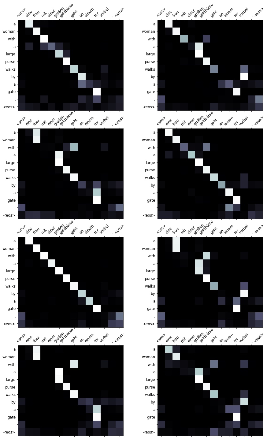
example_idx = 8

src = vars(train_data.examples[example_idx])['src']
trg = vars(train_data.examples[example_idx])['trg']

print(f'src = {src}') # src = ['eine', 'frau', 'mit', 'einer', 'großen', 'geldbörse', 'geht', 'an', 'einem', 'tor', 'vorbei', '.']
print(f'trg = {trg}') # trg = ['a', 'woman', 'with', 'a', 'large', 'purse', 'is', 'walking', 'by', 'a', 'gate', '.']

translation, attention = translate_sentence(src, SRC, TRG, model, device)

print(f'predicted trg = {translation}')# predicted trg = ['a', 'woman', 'with', 'a', 'large', 'purse', 'walks', 'by', 'a', 'gate', '.', '<eos>']

display_attention(src, translation, attention)
Translation looks pretty good, although model changes is walking by to walks by. The meaning is still the same.
Can see the attention from each head below. Each is certainly different, but it’s difficult (perhaps impossible) to reason about what head has actually learned to pay attention to. Some heads pay full attention to “eine” when translating “a”, some don’t at all, and some do a little. They all seem to follow the similar “downward staircase” pattern and the attention when outputting the last two tokens is equally spread over the final two tokens in the input sentence.
Translates an example in the validation set.
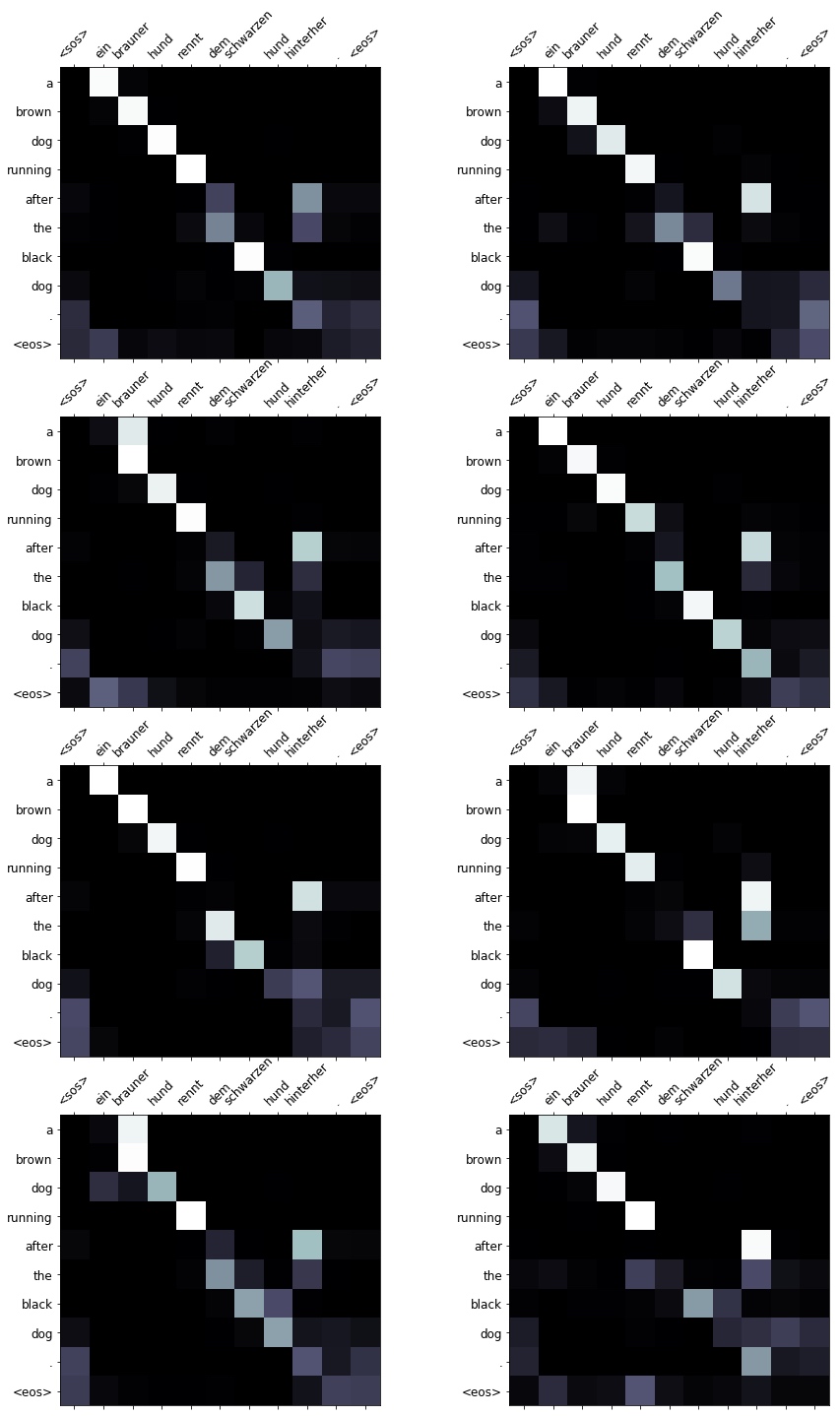
example_idx = 6

src = vars(valid_data.examples[example_idx])['src']
trg = vars(valid_data.examples[example_idx])['trg']

print(f'src = {src}') # src = ['ein', 'brauner', 'hund', 'rennt', 'dem', 'schwarzen', 'hund', 'hinterher', '.']
print(f'trg = {trg}') # trg = ['a', 'brown', 'dog', 'is', 'running', 'after', 'the', 'black', 'dog', '.']

translation, attention = translate_sentence(src, SRC, TRG, model, device)

print(f'predicted trg = {translation}') # predicted trg = ['a', 'brown', 'dog', 'running', 'after', 'the', 'black', 'dog', '.', '<eos>']


display_attention(src, translation, attention)
The model translates it by switching is running to just running, but it is an acceptable swap.
Again, some heads pay full attention to “ein” whilst some pay no attention to it. Again, most of the heads seem to spread their attention over both the period and
Finally, get an example from the test set.
example_idx = 10

src = vars(test_data.examples[example_idx])['src']
trg = vars(test_data.examples[example_idx])['trg']

print(f'src = {src}') # src = ['eine', 'mutter', 'und', 'ihr', 'kleiner', 'sohn', 'genießen', 'einen', 'schönen', 'tag', 'im', 'freien', '.']
print(f'trg = {trg}') # trg = ['a', 'mother', 'and', 'her', 'young', 'song', 'enjoying', 'a', 'beautiful', 'day', 'outside', '.']

translation, attention = translate_sentence(src, SRC, TRG, model, device)

print(f'predicted trg = {translation}') # predicted trg = ['a', 'mother', 'and', 'her', 'son', 'enjoying', 'a', 'beautiful', 'day', 'outside', '.', '<eos>']

display_attention(src, translation, attention)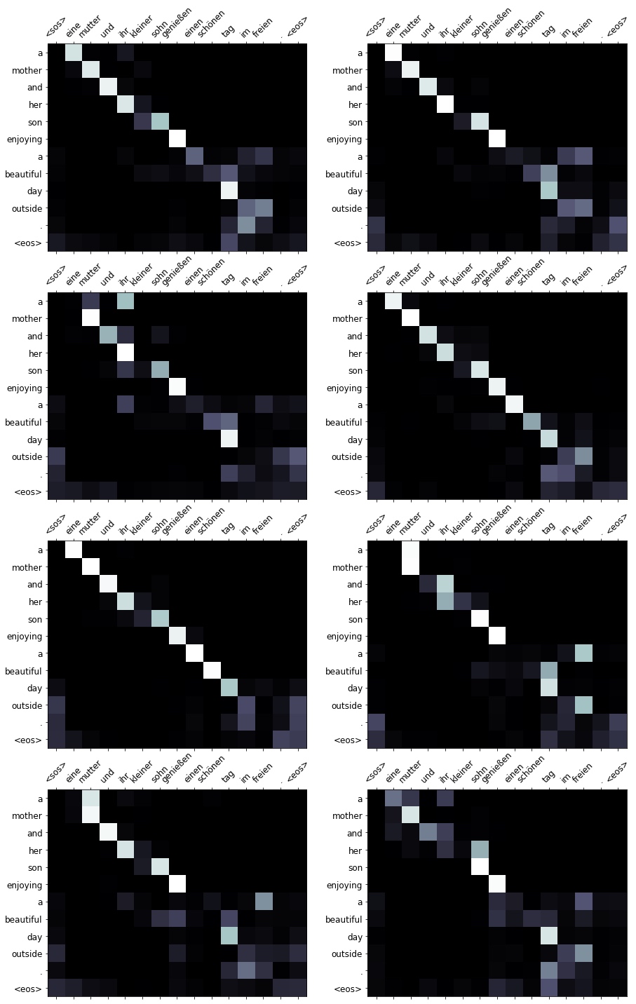
BLEU
Finally, calculate the BLEU score for the model.
from torchtext.data.metrics import bleu_score

def calculate_bleu(data, src_field, trg_field, model, device, max_len = 50):

    trgs = []
    pred_trgs = []

    for datum in data:

        src = vars(datum)['src']
        trg = vars(datum)['trg']

        pred_trg, _ = translate_sentence(src, src_field, trg_field, model, device, max_len)

        #cut off <eos> token
        pred_trg = pred_trg[:-1]

        pred_trgs.append(pred_trg)
        trgs.append([trg])

    return bleu_score(pred_trgs, trgs)
Get a BLEU score of 35.08, which beats the 33.3 of the convolutional sequence-to-sequence model and 28.2 of the attention based RNN model. All this whilst having the least amount of parameters and the fastest training time!
bleu_score = calculate_bleu(test_data, SRC, TRG, model, device)

print(f'BLEU score = {bleu_score*100:.2f}') # BLEU score = 35.08
The end~