3 - Neural Machine Translation by Jointly Learning to Align and Translate
3 - Neural Machine Translation by Jointly Learning to Align and Translate
This part will learn about attention by implementing the model from Neural Machine Translation by Jointly Learning to Align and Translate.
Introduction
In the previous model, architecture was set-up in a way to reduce “information compression” by explicitly passing the context vector, $z$, to the decoder at every time-step and by passing both the context vector and embedded input word, $d(y_t)$, along with the hidden state, $s_t$, to the linear layer, $f$, to make a prediction.
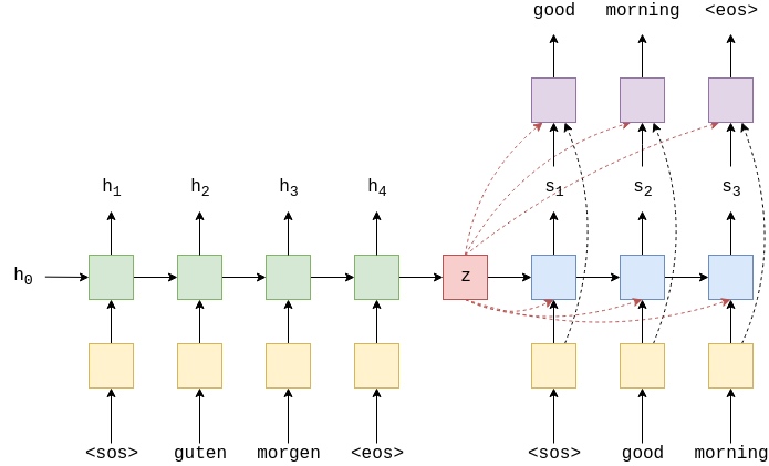
Even though it has reduced some of this compression, context vector still needs to contain all of the information about the source sentence. The model implemented in this part avoids this compression by allowing the decoder to look at the entire source sentence (via its hidden states) at each decoding step by leveraging attention.
Attention works by first, calculating an attention vector, $a$, that is the length of the source sentence. The attention vector has the property that each element is between 0 and 1, and the entire vector sums to 1. Then calculate a weighted sum of our source sentence hidden states, $H$, to get a weighted source vector, $w$.
$$w = \sum_{i}a_ih_i$$
Calculate a new weighted source vector every time-step when decoding, using it as input to decoder RNN as well as the linear layer to make a prediction.
Preparing Data
import torch
import torch.nn as nn
import torch.optim as optim
import torch.nn.functional as F

from torchtext.datasets import TranslationDataset, Multi30k
from torchtext.data import Field, BucketIterator

import spacy
import numpy as np

import random
import math
import time

SEED = 1234

random.seed(SEED)
np.random.seed(SEED)
torch.manual_seed(SEED)
torch.cuda.manual_seed(SEED)
torch.backends.cudnn.deterministic = True

spacy_de = spacy.load('de')
spacy_en = spacy.load('en')

# create tokenizer
def tokenize_de(text):
    """
    Tokenizes German text from a string into a list of strings
    """
    return [tok.text for tok in spacy_de.tokenizer(text)]

def tokenize_en(text):
    """
    Tokenizes English text from a string into a list of strings
    """
    return [tok.text for tok in spacy_en.tokenizer(text)]

# create field
SRC = Field(tokenize=tokenize_de,
            init_token='<sos>',
            eos_token='<eos>',
            lower=True)

TRG = Field(tokenize = tokenize_en,
            init_token='<sos>',
            eos_token='<eos>',
            lower=True)

# Load data
train_data, valid_data, test_data = Multi30k.splits(exts = ('.de', '.en'), fields = (SRC, TRG))
print(vars(train_data.examples[0]))
# {'src': ['zwei', 'junge', 'weiße', 'männer', 'sind', 'im', 'freien', 'in', 'der', 'nähe', 'vieler', 'büsche', '.'], 'trg': ['two', 'young', ',', 'white', 'males', 'are', 'outside', 'near', 'many', 'bushes', '.']}

# Build the vocabulary
SRC.build_vocab(train_data, min_freq = 2)
TRG.build_vocab(train_data, min_freq = 2)

# Define the device and create iterators
device = torch.device('cuda' if torch.cuda.is_available() else 'cpu')

BATCH_SIZE = 128

train_iterator, valid_iterator, test_iterator = BucketIterator.splits(
    (train_data, valid_data, test_data),
    batch_size = BATCH_SIZE,
    device = device)
Building the Seq2Seq Model
Encoder
First, build the encoder. Only use a single layer GRU, however now will use a bidirectional RNN which have two RNNs in each layer. A forward RNN going over the embedded sentence from left to right (shown below in green), and a backward RNN going over the embedded sentence from right to left (shown below in teal). In code, only need to set bidirectional = True and then pass the embedded sentence to the RNN as before.
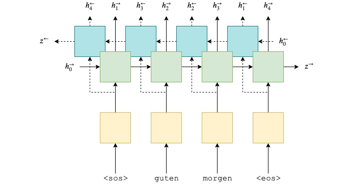
So now have:
$$\begin{align*}
h_t^\rightarrow = \text{EncoderGRU}^\rightarrow(e(x_t^\rightarrow),h_{t-1}^\rightarrow)\\
h_t^\leftarrow = \text{EncoderGRU}^\leftarrow(e(x_t^\leftarrow),h_{t-1}^\leftarrow)
\end{align*}$$
Where $x_0^\rightarrow = \text{<sos>}, x_1^\rightarrow = \text{guten}$ and $x_0^\leftarrow = \text{<eos>}, x_1^\leftarrow = \text{morgen}$.
As before, only pass an input (embedded) to the RNN, which tells PyTorch to initialize both the forward and backward initial hidden states ($h_0^\rightarrow$ and $h_0^\leftarrow$, respectively) to a tensor of all zeros. Also will get two context vectors, one from the forward RNN after it has seen the final word in the sentence, $z^\rightarrow=h_T^\rightarrow$, and one from the backward RNN after it has seen the first word in the sentence, $z^\leftarrow=h_T^\leftarrow$.
The RNN returns outputs and hidden.
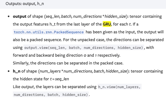
outputsis of size[src len, batch size, hid dim * num directions]where the firsthid_dimelements in the third axis are the hidden states from the top layer forward RNN, and the lasthid_dimelements are hidden states from the top layer backward RNN. The third axis can be regarded as being the forward and backward hidden states concatenated together other, i.e.$h_1 = [h_1^\rightarrow; h_{T}^\leftarrow]$,$h_2 = [h_2^\rightarrow; h_{T-1}^\leftarrow]$and can denote all encoder hidden states (forward and backwards concatenated together) as$H=\{ h_1, h_2, ..., h_T\}$.hiddenis of size[n layers * num directions, batch size, hid dim], where**[-2, :, :]gives the top layer forward RNN hidden state after the final time-step** (i.e. after it has seen the last word in the sentence) and[-1, :, :]gives the top layer backward RNN hidden state after the final time-step (i.e. after it has seen the first word in the sentence).
As the decoder is not bidirectional, it only needs a single context vector, $z$, to use as its initial hidden state, $s_0$, and currently have two, a forward and a backward one ($z^\rightarrow=h_T^\rightarrow$ and $z^\leftarrow=h_T^\leftarrow$, respectively). Can solve this by concatenating the two context vectors together, passing them through a linear layer, $g$, and applying the $\tanh$ activation function.
$$z=\tanh(g(h_T^\rightarrow, h_T^\leftarrow)) = \tanh(g(z^\rightarrow, z^\leftarrow)) = s_0$$
Note: this is actually a deviation from the paper. Instead, they feed only the first backward RNN hidden state through a linear layer to get the context vector/decoder initial hidden state(But seems doesn’t make sense).
Output of GRU:
Output of LSTM: 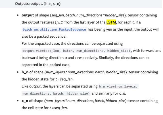
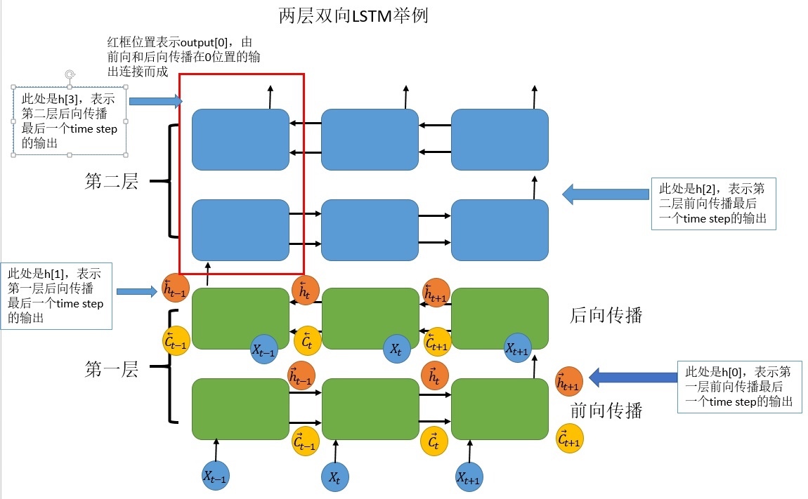
- output保存了最后一层,每个time step的输出h,如果是双向LSTM,每个time step的输出h = [h正向, h逆向] (同一个time step的正向和逆向的h连接起来)
- output是一个三维的张量,第一维表示序列长度,第二维表示一批的样本数(batch),第三维是 hidden_size(隐藏层大小) * num_directions
- num_directions根据”biredirectional=False”取值为1或2
- 如果不是双向,第三个维度等于定义的隐藏层大小,num_directions=1; 如果是双向的,第三个维度的大小等于2倍的隐藏层大小, num_directions=2, 相当于num_layers=2
- h_n保存了每一层,最后一个time step的输出h,如果是双向LSTM,单独保存前向和后向的最后一个time step的输出h
- h_n是一个三维的张量,第一维是num_layers*num_directions; 第二维表示一批的样本数量(batch); 第三维表示隐藏层的大小
- c_n与h_n一致,只是它保存的是c的值
- ref: https://zhuanlan.zhihu.com/p/39191116
例子:
import torch
import torch.nn as nn

bilstm = nn.LSTM(input_size=10, hidden_size=20, num_layers=2, bidirectional=True)
input = torch.randn(5, 3, 10) # sequence length为5,batch size为3,input size为10
h0 = torch.randn(4, 3, 20) # (num_layers * 2, batch, hidden_size) = (4, 3, 20)
c0 = torch.randn(4, 3, 20) # (num_layers * 2, batch, hidden_size) = (4, 3, 20)
output, (hn, cn) = bilstm(input, (h0, c0))

print('output shape: ', output.shape)  # torch.Size([5, 3, 40]) shape (seq_len, batch, num_directions * hidden_size)
print('hn shape: ', hn.shape)  # torch.Size([4, 3, 20]) shape (num_layers * num_directions, batch, hidden_size)
print('cn shape: ', cn.shape)  # torch.Size([4, 3, 20]) shape (num_layers * num_directions, batch, hidden_size)

# 相当于lstm有4层, forward1, backward1,forward2, backward2
print('前向传播时,output中最后一个time step的前20个与hn最后一层前向传播的输出应该一致: ')
print(output[4, 0, :20] == hn[2, 0])
# 4就是最后一个time step, 0就是第一个batch, :20代表前20个, 即为前向传播的h
# 2就是forward2层, 0就是第一个batch, 其所有的h
print('后向传播时,output中最后一个time step的后20个与hn最后一层后向传播的输出应该一致: ')
print(output[0, 0, 20:] == hn[3, 0])
# 0就是第一个time step, 0就是第一个batch, 20:代表后20个h, 即为前向传播的h
# 3就是backward2层, 0就是第一个batch, 其所有的h
这个tutorial用到attention, 所以Encoder的输出除了hidden state(每一层最后一个time step的输出hidden state)还有output(最后一层process每个token时(即每个time step)得到的hidden state的叠加, i.e.$H=\{ h_1, h_2, ..., h_T\}$, 其中,例如$h_1$又是该token前向和后项的hidden state的叠加).将最后一层的前向和后向的最后time step的hidden state叠加, 放到全连接层, fc, 然后使用tanh激活函数, 将其作为hidden返回. (全连接就是矩阵向量乘积y=Wx, 用于对前面特征做加权和 (也类似起到”分类器”的作用))
class Encoder(nn.Module):
    def __init__(self, input_dim, emb_dim, enc_hid_dim, dec_hid_dim, dropout):
        super().__init__()

        self.embedding = nn.Embedding(input_dim, emb_dim)

        self.rnn = nn.GRU(emb_dim, enc_hid_dim, bidirectional = True)

        self.fc = nn.Linear(enc_hid_dim * 2, dec_hid_dim)

        self.dropout = nn.Dropout(dropout)

    def forward(self, src):

        #src = [src len, batch size]

        embedded = self.dropout(self.embedding(src))

        #embedded = [src len, batch size, emb dim]

        outputs, hidden = self.rnn(embedded)

        #outputs = [src len, batch size, hid dim * num directions]
        #hidden = [n layers * num directions, batch size, hid dim]

        #hidden is stacked [forward_1, backward_1, forward_2, backward_2, ...]
        #outputs are always from the last layer
        #hidden [-2, :, : ] is the last of the forwards RNN
        #hidden [-1, :, : ] is the last of the backwards RNN

        #initial decoder hidden is final hidden state of the forwards and backwards
        # encoder RNNs fed through a linear layer
        hidden = torch.tanh(self.fc(torch.cat((hidden[-2,:,:], hidden[-1,:,:]), dim = 1)))
        # 将最后一层的前向和后向的最后time step的hidden state叠加(将所有hid dim叠加在同一维)

        #outputs = [src len, batch size, enc hid dim * 2]
        #hidden = [batch size, dec hid dim]

        return outputs, hidden
Attention
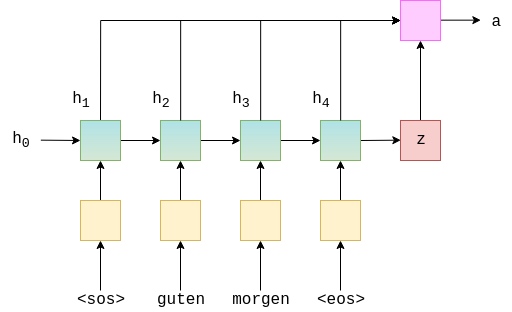
Next up is the attention layer. This will take in the previous hidden state of the decoder, $s_{t-1}$, and all of the stacked forward and backward hidden states from the encoder, $H$. The layer will output an attention vector, $a_t$, that is the length of the source sentence, each element is between 0 and 1 and the entire vector sums to 1.
Intuitively, this layer takes what have decoded so far, $s_{t-1}$, and all of what have encoded, $H$, to produce a vector, $a_t$, that represents which words in the source sentence(german) it should pay the most attention to in order to correctly predict the next word to decode, $\hat{y}_{t+1}$.
First, calculate the energy, $E_t$ between the previous decoder hidden state and the encoder hidden states.
There are three ways to calculate energy (which is the score shown in the below)
 Here, use the third method to retrieve energy score. (concat)
As encoder hidden states are a sequence of $T$ tensors, and previous decoder hidden state is a single tensor, the first thing to do is repeat the previous decoder hidden state $T$ times. Then calculate the energy, $E_t$, between them by concatenating them together and passing them through a linear layer (attn) and a $\tanh$ activation function.
$$E_t = \tanh(\text{attn}(s_{t-1}, H))$$
This can be thought of as calculating how well each encoder hidden state “matches” the previous decoder hidden state.
Currently have a [dec hid dim, src len] tensor for each example in the batch. Need to convert this into [src len] for each example in the batch as the attention should be over the length of the source sentence. This is achieved by multiplying the energy by a [1, dec hid dim] tensor, $v$.
$$\hat{a}_t = v E_t$$
$v$ can be regarded as the weights for a weighted sum of the energy across all encoder hidden states. These weights tell how much it should attend to each token in the source sequence. The parameters of $v$ are initialized randomly, but learned with the rest of the model via backpropagation. Note how $v$ is not dependent on time, and the same $v$ is used for each time-step of the decoding. Implement $v$ as a linear layer without a bias.
Finally, ensure the attention vector, $a_t$ fits the constraints of having all elements between 0 and 1 and the vector summing to 1 by passing it through a $\text{softmax}$ layer.
$$a_t = \text{softmax}(\hat{a_t})$$
This gives the attention over the source sentence!
Graphically, this looks something like below. This is for calculating the very first attention vector, where $s_{t-1} = s_0 = z$. The green/teal blocks represent the hidden states from both the forward and backward RNNs, and the attention computation is all done within the pink block.
class Attention(nn.Module):
    def __init__(self, enc_hid_dim, dec_hid_dim):
        super().__init__()

        self.attn = nn.Linear((enc_hid_dim * 2) + dec_hid_dim, dec_hid_dim)
        self.v = nn.Linear(dec_hid_dim, 1, bias = False)

    def forward(self, hidden, encoder_outputs):

        #hidden = [batch size, dec hid dim]
        #encoder_outputs = [src len, batch size, enc hid dim * 2]

        batch_size = encoder_outputs.shape[1]
        src_len = encoder_outputs.shape[0]

        #repeat decoder hidden state src_len times to match with all hidden state from encoder
        hidden = hidden.unsqueeze(1).repeat(1, src_len, 1)

        encoder_outputs = encoder_outputs.permute(1, 0, 2)

        #hidden = [batch size, src len, dec hid dim]
        #encoder_outputs = [batch size, src len, enc hid dim * 2]

        energy = torch.tanh(self.attn(torch.cat((hidden, encoder_outputs), dim = 2)))

        #energy = [batch size, src len, dec hid dim]

        attention = self.v(energy).squeeze(2) # [batch size, src len, 1] ==> [batch size, src len]

        #attention= [batch size, src len]

        return F.softmax(attention, dim=1)
Decoder
The decoder contains the attention layer, attention, which takes the previous hidden state, $s_{t-1}$, all of the encoder hidden states, $H$, and returns the attention vector, $a_t$.
Then use this attention vector to create a weighted source vector, $w_t$, denoted by weighted, which is a weighted sum of the encoder hidden states, $H$, using $a_t$ as the weights.
$$w_t = a_t H$$
The embedded input word, $d(y_t)$, the weighted source vector, $w_t$, and the previous decoder hidden state, $s_{t-1}$, are then all passed into the decoder RNN, with $d(y_t)$ and $w_t$ being concatenated together.
$$s_t = \text{DecoderGRU}(d(y_t), w_t, s_{t-1})$$
Then pass $d(y_t)$, $w_t$ and $s_t$ through the linear layer, $f$, to make a prediction of the next word in the target sentence, $\hat{y}_{t+1}$. This is done by concatenating them all together.
$$\hat{y}_{t+1} = f(d(y_t), w_t, s_t)$$
The image below shows decoding the first word in an example translation.
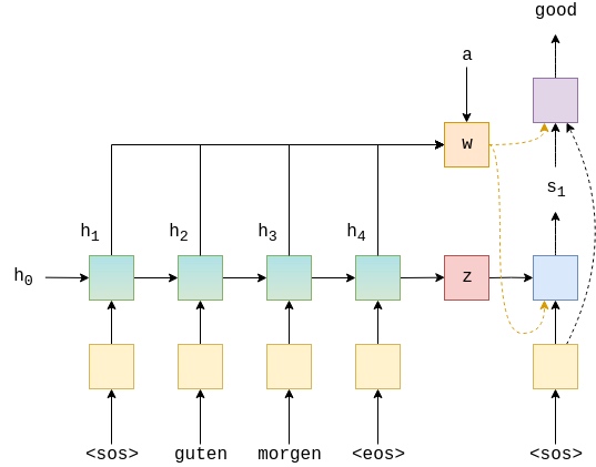
The green/teal(Gradient color one) blocks show the forward/backward encoder RNNs which output $H$, the red block shows the context vector, $z = h_T = \tanh(g(h^\rightarrow_T,h^\leftarrow_T)) = \tanh(g(z^\rightarrow, z^\leftarrow)) = s_0$, the blue block shows the decoder RNN which outputs $s_t$, the purple block shows the linear layer, $f$, which outputs $\hat{y}_{t+1}$ and the orange block shows the calculation of the weighted sum over $H$(all encoder hidden state) by $a_t$(weight) and outputs $w_t$(weighted vector). Not shown is the calculation of $a_t$.
class Decoder(nn.Module):
    def __init__(self, output_dim, emb_dim, enc_hid_dim, dec_hid_dim, dropout, attention):
        super().__init__()

        self.output_dim = output_dim
        self.attention = attention

        self.embedding = nn.Embedding(output_dim, emb_dim)

        self.rnn = nn.GRU((enc_hid_dim * 2) + emb_dim, dec_hid_dim)

        self.fc_out = nn.Linear((enc_hid_dim * 2) + dec_hid_dim + emb_dim, output_dim)

        self.dropout = nn.Dropout(dropout)

    def forward(self, input, hidden, encoder_outputs):

        #input = [batch size]
        #hidden = [batch size, dec hid dim]
        #encoder_outputs = [src len, batch size, enc hid dim * 2]

        input = input.unsqueeze(0)

        #input = [1, batch size]

        embedded = self.dropout(self.embedding(input))

        #embedded = [1, batch size, emb dim]

        a = self.attention(hidden, encoder_outputs)

        #a = [batch size, src len]

        a = a.unsqueeze(1)

        #a = [batch size, 1, src len]

        encoder_outputs = encoder_outputs.permute(1, 0, 2)

        #encoder_outputs = [batch size, src len, enc hid dim * 2]

        weighted = torch.bmm(a, encoder_outputs)

        #weighted = [batch size, 1, enc hid dim * 2]

        weighted = weighted.permute(1, 0, 2)

        #weighted = [1, batch size, enc hid dim * 2]

        rnn_input = torch.cat((embedded, weighted), dim = 2)

        #rnn_input = [1, batch size, (enc hid dim * 2) + emb dim]

        output, hidden = self.rnn(rnn_input, hidden.unsqueeze(0))

        #output = [seq len, batch size, dec hid dim * n directions]
        #hidden = [n layers * n directions, batch size, dec hid dim]

        #seq len, n layers and n directions will always be 1 in this decoder, therefore:
        #output = [1, batch size, dec hid dim]
        #hidden = [1, batch size, dec hid dim]
        #this also means that output == hidden
        assert (output == hidden).all() # .all() returns True if all items in an iterable are true

        embedded = embedded.squeeze(0)
        output = output.squeeze(0)
        weighted = weighted.squeeze(0)

        prediction = self.fc_out(torch.cat((output, weighted, embedded), dim = 1))

        #prediction = [batch size, output dim]

        return prediction, hidden.squeeze(0)
Seq2Seq Model
This seq2seq encapsulator is similar to the last two. The only difference is that the encoder returns both the final hidden state(which is the final hidden state from both the forward and backward encoder RNNs passed through a linear layer) to be used as the initial hidden state for the decoder, as well as every hidden state (which are the forward and backward hidden states stacked on top of each other). Also need to ensure that hidden and encoder_outputs are passed to the decoder.
Briefly going over all of the steps:
- the outputs tensor is created to hold all predictions,
$\hat{Y}$ - the source sequence,
$X$, is fed into the encoder to receive$z$and$H$ - the initial decoder hidden state is set to be the context vector,
$s_0 = z = h_T$ - use a batch of
tokens as the first input, $y_1$ - then decode within a loop:
- inserting the input token
$y_t$, previous hidden state,$s_{t-1}$, and all encoder outputs,$H$, into the decoder - receiving a prediction,
$\hat{y}_{t+1}$, and a new hidden state,$s_t$ - then decide if we are going to teacher force or not, setting the next input as appropriate
- inserting the input token
class Seq2Seq(nn.Module):
    def __init__(self, encoder, decoder, device):
        super().__init__()

        self.encoder = encoder
        self.decoder = decoder
        self.device = device

    def forward(self, src, trg, teacher_forcing_ratio = 0.5):

        #src = [src len, batch size]
        #trg = [trg len, batch size]
        #teacher_forcing_ratio is probability to use teacher forcing
        #e.g. if teacher_forcing_ratio is 0.75 we use teacher forcing 75% of the time

        batch_size = src.shape[1]
        trg_len = trg.shape[0]
        trg_vocab_size = self.decoder.output_dim

        #tensor to store decoder outputs
        outputs = torch.zeros(trg_len, batch_size, trg_vocab_size).to(self.device)

        #encoder_outputs is all hidden states of the input sequence, back and forwards
        #hidden is the final forward and backward hidden states, passed through a linear layer
        encoder_outputs, hidden = self.encoder(src)

        #first input to the decoder is the <sos> tokens
        input = trg[0,:]

        for t in range(1, trg_len):

            #insert input token embedding, previous hidden state and all encoder hidden states
            #receive output tensor (predictions) and new hidden state
            output, hidden = self.decoder(input, hidden, encoder_outputs)

            #place predictions in a tensor holding predictions for each token
            outputs[t] = output

            #decide if we are going to use teacher forcing or not
            teacher_force = random.random() < teacher_forcing_ratio

            #get the highest predicted token from our predictions
            top1 = output.argmax(1)

            #if teacher forcing, use actual next token as next input
            #if not, use predicted token
            input = trg[t] if teacher_force else top1

        return outputs
Training the Seq2Seq Model
Initialise encoder, decoder and seq2seq model as before.
INPUT_DIM = len(SRC.vocab)
OUTPUT_DIM = len(TRG.vocab)
ENC_EMB_DIM = 256
DEC_EMB_DIM = 256
ENC_HID_DIM = 512
DEC_HID_DIM = 512
ENC_DROPOUT = 0.5
DEC_DROPOUT = 0.5

attn = Attention(ENC_HID_DIM, DEC_HID_DIM)
enc = Encoder(INPUT_DIM, ENC_EMB_DIM, ENC_HID_DIM, DEC_HID_DIM, ENC_DROPOUT)
dec = Decoder(OUTPUT_DIM, DEC_EMB_DIM, ENC_HID_DIM, DEC_HID_DIM, DEC_DROPOUT, attn)

model = Seq2Seq(enc, dec, device).to(device)
Next, use a simplified version of the weight initialization scheme used in the paper. Here will initialize all biases to zero and all weights from $\mathcal{N}(0, 0.01)$.
def init_weights(m):
    for name, param in m.named_parameters():
        if 'weight' in name:
            nn.init.normal_(param.data, mean=0, std=0.01)
        else:
            nn.init.constant_(param.data, 0)

model.apply(init_weights)
'''
Seq2Seq(
  (encoder): Encoder(
    (embedding): Embedding(7853, 256)
    (rnn): GRU(256, 512, bidirectional=True)
    (fc): Linear(in_features=1024, out_features=512, bias=True)
    (dropout): Dropout(p=0.5, inplace=False)
  )
  (decoder): Decoder(
    (attention): Attention(
      (attn): Linear(in_features=1536, out_features=512, bias=True)
      (v): Linear(in_features=512, out_features=1, bias=False)
    )
    (embedding): Embedding(5893, 256)
    (rnn): GRU(1280, 512)
    (fc_out): Linear(in_features=1792, out_features=5893, bias=True)
    (dropout): Dropout(p=0.5, inplace=False)
  )
)
'''
Calculate the number of parameters. Get an increase of almost 50% in the amount of parameters from the last model.
def count_parameters(model):
    return sum(p.numel() for p in model.parameters() if p.requires_grad)

print(f'The model has {count_parameters(model):,} trainable parameters') # The model has 20,518,405 trainable parameters
Initiaize optimizer and the loss function, making sure to ignore the loss on
optimizer = optim.Adam(model.parameters())

TRG_PAD_IDX = TRG.vocab.stoi[TRG.pad_token]

criterion = nn.CrossEntropyLoss(ignore_index = TRG_PAD_IDX)
Create the training loop and the evaluation loop, remembering to set the model to eval mode and turn off teaching forcing. And create a function that calculates how long an epoch takes
def train(model, iterator, optimizer, criterion, clip):

    model.train()

    epoch_loss = 0

    for i, batch in enumerate(iterator):

        src = batch.src
        trg = batch.trg

        optimizer.zero_grad()

        output = model(src, trg)

        #trg = [trg len, batch size]
        #output = [trg len, batch size, output dim]

        output_dim = output.shape[-1]

        output = output[1:].view(-1, output_dim)
        trg = trg[1:].view(-1)

        #trg = [(trg len - 1) * batch size]
        #output = [(trg len - 1) * batch size, output dim]

        loss = criterion(output, trg)

        loss.backward()

        torch.nn.utils.clip_grad_norm_(model.parameters(), clip)

        optimizer.step()

        epoch_loss += loss.item()

    return epoch_loss / len(iterator)

def evaluate(model, iterator, criterion):

    model.eval()

    epoch_loss = 0

    with torch.no_grad():

        for i, batch in enumerate(iterator):

            src = batch.src
            trg = batch.trg

            output = model(src, trg, 0) #turn off teacher forcing

            #trg = [trg len, batch size]
            #output = [trg len, batch size, output dim]

            output_dim = output.shape[-1]

            output = output[1:].view(-1, output_dim)
            trg = trg[1:].view(-1)

            #trg = [(trg len - 1) * batch size]
            #output = [(trg len - 1) * batch size, output dim]

            loss = criterion(output, trg)

            epoch_loss += loss.item()

    return epoch_loss / len(iterator)

def epoch_time(start_time, end_time):
    elapsed_time = end_time - start_time
    elapsed_mins = int(elapsed_time / 60)
    elapsed_secs = int(elapsed_time - (elapsed_mins * 60))
    return elapsed_mins, elapsed_secs
Train model, saving the parameters that give the best validation loss.
N_EPOCHS = 10
CLIP = 1

best_valid_loss = float('inf')

for epoch in range(N_EPOCHS):

    start_time = time.time()

    train_loss = train(model, train_iterator, optimizer, criterion, CLIP)
    valid_loss = evaluate(model, valid_iterator, criterion)

    end_time = time.time()

    epoch_mins, epoch_secs = epoch_time(start_time, end_time)

    if valid_loss < best_valid_loss:
        best_valid_loss = valid_loss
        torch.save(model.state_dict(), 'tut3-model.pt')

    print(f'Epoch: {epoch+1:02} | Time: {epoch_mins}m {epoch_secs}s')
    print(f'\tTrain Loss: {train_loss:.3f} | Train PPL: {math.exp(train_loss):7.3f}')
    print(f'\t Val. Loss: {valid_loss:.3f} |  Val. PPL: {math.exp(valid_loss):7.3f}')
'''
Epoch: 01 | Time: 0m 57s
	Train Loss: 5.016 | Train PPL: 150.847
	 Val. Loss: 4.910 |  Val. PPL: 135.637
Epoch: 02 | Time: 0m 56s
	Train Loss: 4.126 | Train PPL:  61.952
	 Val. Loss: 4.545 |  Val. PPL:  94.121
Epoch: 03 | Time: 0m 53s
	Train Loss: 3.472 | Train PPL:  32.191
	 Val. Loss: 3.822 |  Val. PPL:  45.718
Epoch: 04 | Time: 0m 54s
	Train Loss: 2.906 | Train PPL:  18.283
	 Val. Loss: 3.451 |  Val. PPL:  31.516
Epoch: 05 | Time: 0m 53s
	Train Loss: 2.501 | Train PPL:  12.196
	 Val. Loss: 3.292 |  Val. PPL:  26.887
Epoch: 06 | Time: 0m 54s
	Train Loss: 2.207 | Train PPL:   9.089
	 Val. Loss: 3.260 |  Val. PPL:  26.037
Epoch: 07 | Time: 0m 53s
	Train Loss: 1.963 | Train PPL:   7.124
	 Val. Loss: 3.186 |  Val. PPL:  24.190
Epoch: 08 | Time: 0m 53s
	Train Loss: 1.746 | Train PPL:   5.734
	 Val. Loss: 3.229 |  Val. PPL:  25.266
Epoch: 09 | Time: 0m 56s
	Train Loss: 1.579 | Train PPL:   4.848
	 Val. Loss: 3.277 |  Val. PPL:  26.486
Epoch: 10 | Time: 0m 55s
	Train Loss: 1.468 | Train PPL:   4.340
	 Val. Loss: 3.321 |  Val. PPL:  27.693
'''
Finally, test the model on the test set using these “best” parameters.
model.load_state_dict(torch.load('tut3-model.pt'))

test_loss = evaluate(model, test_iterator, criterion)

print(f'| Test Loss: {test_loss:.3f} | Test PPL: {math.exp(test_loss):7.3f} |') # | Test Loss: 3.203 | Test PPL:  24.617 |  Better performance than previous one, but this came at the cost of doubling the training time