2 - Learning Phrase Representations using RNN Encoder-Decoder for Statistical Machine Translation
2 - Learning Phrase Representations using RNN Encoder-Decoder for Statistical Machine Translation
This part will be implementing the model from Learning Phrase Representations using RNN Encoder-Decoder for Statistical Machine Translation. This model will achieve improved test perplexity whilst only using a single layer RNN in both the encoder and the decoder.
Introduction
In the previous model, it is used a multi-layered LSTM as the encoder and decoder.
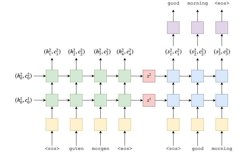
One downside of the previous model is that the decoder is trying to cram lots of information into the hidden states. Whilst decoding, the hidden state will need to contain information about the whole of the source sequence, as well as all of the tokens have been decoded so far. Therefore, this part will implement the paper to alleviate some of this information compression.
This part will also be using a GRU (Gated Recurrent Unit) instead of an LSTM (Long Short-Term Memory). How GRUs (and LSTMs) differ from standard RNNS. Is a GRU better than an LSTM? Research has shown they’re pretty much the same, and both are better than standard RNNs.
Preparing Data
import torch.nn as nn
import torch.optim as optim

from torchtext.datasets import TranslationDataset, Multi30k
from torchtext.data import Field, BucketIterator

import spacy
import numpy as np

import random
import math
import time

SEED = 1234

random.seed(SEED)
np.random.seed(SEED)
torch.manual_seed(SEED)
torch.cuda.manual_seed(SEED)
torch.backends.cudnn.deterministic = True

spacy_de = spacy.load('de')
spacy_en = spacy.load('en')
Previously reversed the source (German) sentence, however in the paper this time, they don’t do this.
def tokenize_de(text):
    """
    Tokenizes German text from a string into a list of strings
    """
    return [tok.text for tok in spacy_de.tokenizer(text)]

def tokenize_en(text):
    """
    Tokenizes English text from a string into a list of strings
    """
    return [tok.text for tok in spacy_en.tokenizer(text)]
Create fields to process our data. This will append the “start of sentence” and “end of sentence” tokens as well as converting all words to lowercase.
SRC = Field(tokenize=tokenize_de,
            init_token='<sos>',
            eos_token='<eos>',
            lower=True)

TRG = Field(tokenize = tokenize_en,
            init_token='<sos>',
            eos_token='<eos>',
            lower=True)
Load data
train_data, valid_data, test_data = Multi30k.splits(exts = ('.de', '.en'), fields = (SRC, TRG))
print(vars(train_data.examples[0]))
# {'src': ['zwei', 'junge', 'weiße', 'männer', 'sind', 'im', 'freien', 'in', 'der', 'nähe', 'vieler', 'büsche', '.'], 'trg': ['two', 'young', ',', 'white', 'males', 'are', 'outside', 'near', 'many', 'bushes', '.']}
Then create our vocabulary, converting all tokens appearing less than twice into
SRC.build_vocab(train_data, min_freq = 2)
TRG.build_vocab(train_data, min_freq = 2)
Define the device and create iterators
device = torch.device('cuda' if torch.cuda.is_available() else 'cpu')

BATCH_SIZE = 128

train_iterator, valid_iterator, test_iterator = BucketIterator.splits(
    (train_data, valid_data, test_data),
    batch_size = BATCH_SIZE,
    device = device)
Building the Seq2Seq Model
Encoder
The encoder is similar to the previous one, with the multi-layer LSTM swapped for a single-layer GRU. Don’t need to pass the dropout as an argument to the GRU as that dropout is used between each layer of a multi-layered RNN.
Another thing to note about the GRU is that it only requires and returns a hidden state, there is no cell state like in the LSTM.
$$\begin{align*}
h_t = \text{GRU}(e(x_t), h_{t-1})\\
(h_t, c_t) = \text{LSTM}(e(x_t), h_{t-1}, c_{t-1})\\
h_t = \text{RNN}(e(x_t), h_{t-1})
\end{align*}$$
From the equations above, it looks like the RNN and the GRU are identical. Inside the GRU, however, is a number of gating mechanisms(update gate) that control the information flow in to and out of the hidden state (similar to an LSTM).
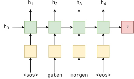
Encoder takes in a sequence, $X = \{x_1, x_2, ... , x_T\}$, passes it through the embedding layer, recurrently calculates hidden states, $H = \{h_1, h_2, ..., h_T\}$, and returns a context vector (the final hidden state), $z=h_T$.
$$h_t = \text{EncoderGRU}(e(x_t), h_{t-1})$$
This is identical to the encoder of the general seq2seq model, with all the “magic” happening inside the GRU (green).
class Encoder(nn.Module):
    def __init__(self, input_dim, emb_dim, hid_dim, dropout):
        super().__init__()

        self.hid_dim = hid_dim

        self.embedding = nn.Embedding(input_dim, emb_dim) # no dropout as only one layer!

        self.rnn = nn.GRU(emb_dim, hid_dim)

        self.dropout = nn.Dropout(dropout)

    def forward(self, src):

        #src = [src len, batch size]

        embedded = self.dropout(self.embedding(src))

        #embedded = [src len, batch size, emb dim]

        outputs, hidden = self.rnn(embedded) #no cell state!

        #outputs = [src len, batch size, hid dim * n directions]
        #hidden = [n layers * n directions, batch size, hid dim]

        #outputs are always from the top hidden layer

        return hidden
Decoder
The decoder is where the implementation differs significantly from the previous model and alleviate some of the information compression.
Instead of the GRU in the decoder taking just the embedded target token, $d(y_t)$ and the previous hidden state $s_{t-1}$ as inputs, it also takes the context vector $z$.
$$s_t = \text{DecoderGRU}(d(y_t), s_{t-1}, z)$$
Note how this context vector, $z$, does not have a $t$ subscript, meaning that re-use the same context vector returned by the encoder for every time-step in the decoder.
In last tutorial, it predicted the next token, $\hat{y}_{t+1}$, with the linear layer(purple part), $f$, only using the top-layer decoder hidden state at that time-step, $s_t$, as $\hat{y}_{t+1}=f(s_t^L)$. In this tutorial, it also pass the embedding of current token, $d(y_t)$ and the context vector, $z$ to the linear layer.
$$\hat{y}_{t+1} = f(d(y_t), s_t, z)$$
Thus, decoder now looks something like this:
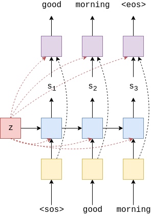
Note, the initial hidden state, $s_0$, is still the context vector, $z$, so when generating the first token, it is actually inputting two identical context vectors into the GRU.(when generating the first token)
How do these two changes reduce the information compression? Hypothetically the decoder hidden states, $s_t$, no longer need to contain information about the source sequence as it is always available as an input. Thus, it only needs to contain information about what tokens it has generated so far. The addition of $y_t$ to the linear layer also means this layer can directly see what the token is, without having to get this information from the hidden state.
However, it is just a hypothesis, it is impossible to determine how the model actually uses the information provided to it. Nevertheless, it is a solid intuition and the results seem to indicate that this modifications are a good idea.
Within the implementation(forward function), pass $d(y_t)$ and $z$ to the GRU by concatenating them together as emb_con, so the input dimensions to the GRU are now emb_dim + hid_dim (as context vector will be of size hid_dim). The linear layer will take $d(y_t), s_t$ and $z$ also by concatenating them together, hence the input dimensions are now emb_dim + hid_dim*2, feeding it through the linear layer to receive predictions, $\hat{y}_{t+1}$.
跟上一个教程的差别就是, 这里用的是GRU而不是LSTM. 最重要的一点是, 每次Decoder都会输入Encoder输出的cotext vector. 一开始将word emb 跟 cotext vector concat到一起, 然后输入到GRU; 再将GRU输出的output, hidden state 和 cotext vector concat到一起, 然后输入到全连接层得到最后output, 其shape为[batch size, emb dim + hid dim * 2]
class Decoder(nn.Module):
    def __init__(self, output_dim, emb_dim, hid_dim, dropout):
        super().__init__()

        self.hid_dim = hid_dim
        self.output_dim = output_dim

        self.embedding = nn.Embedding(output_dim, emb_dim)

        self.rnn = nn.GRU(emb_dim + hid_dim, hid_dim)

        self.fc_out = nn.Linear(emb_dim + hid_dim * 2, output_dim)

        self.dropout = nn.Dropout(dropout)

    def forward(self, input, hidden, context):

        #input = [batch size]
        #hidden = [n layers * n directions, batch size, hid dim]
        #context = [n layers * n directions, batch size, hid dim]

        #n layers and n directions in the decoder will both always be 1, therefore:
        #hidden = [1, batch size, hid dim]
        #context = [1, batch size, hid dim]

        input = input.unsqueeze(0)

        #input = [1, batch size]

        embedded = self.dropout(self.embedding(input))

        #embedded = [1, batch size, emb dim]

        emb_con = torch.cat((embedded, context), dim = 2) # 将所有的 emb dim 和 hid dim 叠加在同一维

        #emb_con = [1, batch size, emb dim + hid dim]

        output, hidden = self.rnn(emb_con, hidden)

        #output = [seq len, batch size, hid dim * n directions]
        #hidden = [n layers * n directions, batch size, hid dim]

        #seq len, n layers and n directions will always be 1 in the decoder, therefore:
        #output = [1, batch size, hid dim]
        #hidden = [1, batch size, hid dim]

        output = torch.cat((embedded.squeeze(0), hidden.squeeze(0), context.squeeze(0)), dim = 1) # 将embedded,hidden,context全部去掉第1维, 然后将这三个的hid dim叠加在同一维

        #output = [batch size, emb dim + hid dim * 2]

        prediction = self.fc_out(output)

        #prediction = [batch size, output dim]

        return prediction, hidden
Seq2Seq Model
Putting the encoder and decoder together, can get:
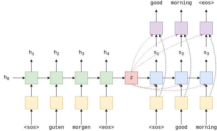
Again, in this implementation, need to ensure the hidden dimensions in both the encoder and the decoder are the same.
Briefly going over all of the steps:
- the outputs tensor is created to hold all predictions,
$\hat{Y}$ - the source sequence,
$X$, is fed into the encoder to receive a context vector - the initial decoder hidden state is set to be the context vector,
$s_0 = z = h_T$ - use a batch of
tokens as the first input, $y_1$ - then decode within a loop:
- inserting the input token
$y_t$, previous hidden state,$s_{t-1}$, and the context vector,$z$, into the decoder - receiving a prediction,
$\hat{y}_{t+1}$, and a new hidden state,$s_t$ then decide if use teacher force or not, setting the next input as appropriate (either the ground truth next token in the target sequence or the highest predicted next token)
class Seq2Seq(nn.Module):
def __init__(self, encoder, decoder, device):
    super().__init__()

    self.encoder = encoder
    self.decoder = decoder
    self.device = device

    assert encoder.hid_dim == decoder.hid_dim, \
        "Hidden dimensions of encoder and decoder must be equal!"

def forward(self, src, trg, teacher_forcing_ratio = 0.5):

    #src = [src len, batch size]
    #trg = [trg len, batch size]
    #teacher_forcing_ratio is probability to use teacher forcing
    #e.g. if teacher_forcing_ratio is 0.75 we use ground-truth inputs 75% of the time

    batch_size = trg.shape[1]
    trg_len = trg.shape[0]
    trg_vocab_size = self.decoder.output_dim

    #tensor to store decoder outputs
    outputs = torch.zeros(trg_len, batch_size, trg_vocab_size).to(self.device)

    #last hidden state of the encoder is the context
    context = self.encoder(src)

    #context also used as the initial hidden state of the decoder
    hidden = context

    #first input to the decoder is the <sos> tokens
    input = trg[0,:]

    for t in range(1, trg_len):

        #insert input token embedding, previous hidden state and the context state
        #receive output tensor (predictions) and new hidden state
        output, hidden = self.decoder(input, hidden, context)

        #place predictions in a tensor holding predictions for each token
        outputs[t] = output

        #decide if we are going to use teacher forcing or not
        teacher_force = random.random() < teacher_forcing_ratio

        #get the highest predicted token from our predictions
        top1 = output.argmax(1)

        #if teacher forcing, use actual next token as next input
        #if not, use predicted token
        input = trg[t] if teacher_force else top1

    return outputs
Training the Seq2Seq Model
Initialise encoder, decoder and seq2seq model. As before, the embedding dimensions and the amount of dropout used can be different between the encoder and the decoder, but the hidden dimensions must remain the same.
INPUT_DIM = len(SRC.vocab)
OUTPUT_DIM = len(TRG.vocab)
ENC_EMB_DIM = 256
DEC_EMB_DIM = 256
HID_DIM = 512
ENC_DROPOUT = 0.5
DEC_DROPOUT = 0.5

enc = Encoder(INPUT_DIM, ENC_EMB_DIM, HID_DIM, ENC_DROPOUT)
dec = Decoder(OUTPUT_DIM, DEC_EMB_DIM, HID_DIM, DEC_DROPOUT)

device = torch.device('cuda' if torch.cuda.is_available() else 'cpu')

model = Seq2Seq(enc, dec, device).to(device)
Next, initialize parameters. The paper states the parameters are initialized from a normal distribution with a mean of 0 and a standard deviation of 0.01, i.e. $\mathcal{N}(0, 0.01)$.
def init_weights(m):
    for name, param in m.named_parameters():
        nn.init.normal_(param.data, mean=0, std=0.01)

model.apply(init_weights)
'''
Seq2Seq(
  (encoder): Encoder(
    (embedding): Embedding(7855, 256)
    (rnn): GRU(256, 512)
    (dropout): Dropout(p=0.5, inplace=False)
  )
  (decoder): Decoder(
    (embedding): Embedding(5893, 256)
    (rnn): GRU(768, 512)
    (fc_out): Linear(in_features=1280, out_features=5893, bias=True)
    (dropout): Dropout(p=0.5, inplace=False)
  )
)
'''
Print out the number of parameters.
Even though only have a single layer RNN for encoder and decoder ,it is actually have more parameters than the last model. This is due to the increased size of the inputs to the GRU and the linear layer. However, it is not a significant amount of parameters and causes a minimal amount of increase in training time (~3 seconds per epoch extra).
def count_parameters(model):
    return sum(p.numel() for p in model.parameters() if p.requires_grad)

print(f'The model has {count_parameters(model):,} trainable parameters') # The model has 14,220,293 trainable parameters
Initiaize optimizer and the loss function, making sure to ignore the loss on
optimizer = optim.Adam(model.parameters())

TRG_PAD_IDX = TRG.vocab.stoi[TRG.pad_token]

criterion = nn.CrossEntropyLoss(ignore_index = TRG_PAD_IDX)
Create the training loop and the evaluation loop, remembering to set the model to eval mode and turn off teaching forcing. And create a function that calculates how long an epoch takes
def train(model, iterator, optimizer, criterion, clip):

    model.train()

    epoch_loss = 0

    for i, batch in enumerate(iterator):

        src = batch.src
        trg = batch.trg

        optimizer.zero_grad()

        output = model(src, trg)

        #trg = [trg len, batch size]
        #output = [trg len, batch size, output dim]

        output_dim = output.shape[-1]

        output = output[1:].view(-1, output_dim)
        trg = trg[1:].view(-1)

        #trg = [(trg len - 1) * batch size]
        #output = [(trg len - 1) * batch size, output dim]

        loss = criterion(output, trg)

        loss.backward()

        torch.nn.utils.clip_grad_norm_(model.parameters(), clip)

        optimizer.step()

        epoch_loss += loss.item()

    return epoch_loss / len(iterator)

def evaluate(model, iterator, criterion):

    model.eval()

    epoch_loss = 0

    with torch.no_grad():

        for i, batch in enumerate(iterator):

            src = batch.src
            trg = batch.trg

            output = model(src, trg, 0) #turn off teacher forcing

            #trg = [trg len, batch size]
            #output = [trg len, batch size, output dim]

            output_dim = output.shape[-1]

            output = output[1:].view(-1, output_dim)
            trg = trg[1:].view(-1)

            #trg = [(trg len - 1) * batch size]
            #output = [(trg len - 1) * batch size, output dim]

            loss = criterion(output, trg)

            epoch_loss += loss.item()

    return epoch_loss / len(iterator)

def epoch_time(start_time, end_time):
    elapsed_time = end_time - start_time
    elapsed_mins = int(elapsed_time / 60)
    elapsed_secs = int(elapsed_time - (elapsed_mins * 60))
    return elapsed_mins, elapsed_secs
Train model, saving the parameters that give the best validation loss.
N_EPOCHS = 10
CLIP = 1

best_valid_loss = float('inf')

for epoch in range(N_EPOCHS):

    start_time = time.time()

    train_loss = train(model, train_iterator, optimizer, criterion, CLIP)
    valid_loss = evaluate(model, valid_iterator, criterion)

    end_time = time.time()

    epoch_mins, epoch_secs = epoch_time(start_time, end_time)

    if valid_loss < best_valid_loss:
        best_valid_loss = valid_loss
        torch.save(model.state_dict(), 'tut2-model.pt')

    print(f'Epoch: {epoch+1:02} | Time: {epoch_mins}m {epoch_secs}s')
    print(f'\tTrain Loss: {train_loss:.3f} | Train PPL: {math.exp(train_loss):7.3f}')
    print(f'\t Val. Loss: {valid_loss:.3f} |  Val. PPL: {math.exp(valid_loss):7.3f}')
'''
Epoch: 01 | Time: 0m 26s
	Train Loss: 5.078 | Train PPL: 160.492
	 Val. Loss: 5.280 |  Val. PPL: 196.439
Epoch: 02 | Time: 0m 26s
	Train Loss: 4.399 | Train PPL:  81.332
	 Val. Loss: 5.145 |  Val. PPL: 171.603
Epoch: 03 | Time: 0m 26s
	Train Loss: 4.055 | Train PPL:  57.698
	 Val. Loss: 4.728 |  Val. PPL: 113.078
Epoch: 04 | Time: 0m 26s
	Train Loss: 3.665 | Train PPL:  39.049
	 Val. Loss: 4.349 |  Val. PPL:  77.383
Epoch: 05 | Time: 0m 26s
	Train Loss: 3.319 | Train PPL:  27.631
	 Val. Loss: 4.073 |  Val. PPL:  58.740
Epoch: 06 | Time: 0m 26s
	Train Loss: 3.031 | Train PPL:  20.719
	 Val. Loss: 3.862 |  Val. PPL:  47.564
Epoch: 07 | Time: 0m 26s
	Train Loss: 2.792 | Train PPL:  16.316
	 Val. Loss: 3.711 |  Val. PPL:  40.882
Epoch: 08 | Time: 0m 25s
	Train Loss: 2.551 | Train PPL:  12.822
	 Val. Loss: 3.619 |  Val. PPL:  37.295
Epoch: 09 | Time: 0m 26s
	Train Loss: 2.337 | Train PPL:  10.345
	 Val. Loss: 3.647 |  Val. PPL:  38.377
Epoch: 10 | Time: 0m 25s
	Train Loss: 2.179 | Train PPL:   8.840
	 Val. Loss: 3.602 |  Val. PPL:  36.660
'''
Finally, test the model on the test set using these “best” parameters.
model.load_state_dict(torch.load('tut2-model.pt'))

test_loss = evaluate(model, test_iterator, criterion)

print(f'| Test Loss: {test_loss:.3f} | Test PPL: {math.exp(test_loss):7.3f} |') # | Test Loss: 3.551 | Test PPL:  34.853 |  Better performance than previous one
Save to gdrive
from google.colab import drive
drive.mount('/content/gdrive')

model_save_name = 'tut2-model.pt'
path = F"/content/gdrive/My Drive/{model_save_name}"
torch.save(model.state_dict(), path)
Translate sentence
def translate_sentence(sentence,src_field,trg_field,model,device, max_len=50):
    model.eval()

    if isinstance(sentence,str):
        nlp = spacy.load('de')
        tokens = [token.text.lower() for token in nlp(sentence)]
    else:
        tokens = [token.lower() for token in sentence]

    tokens = [src_field.init_token] + tokens + [src_field.eos_token]

    src_indexes = [src_field.vocab.stoi[token] for token in tokens]
    src_tensor = torch.LongTensor(src_indexes).unsqueeze(1).to(device)

    with torch.no_grad():
        context = model.encoder(src_tensor)

    trg_indexes = [trg_field.vocab.stoi[trg_field.init_token]] #<sos>
    hidden = context

    for i in range(max_len):
        trg_tensor = torch.LongTensor([trg_indexes[-1]]).to(device)

        with torch.no_grad():
            output, hidden = model.decoder(trg_tensor, hidden, context)
        pred_token = output.argmax(1).item()
        trg_indexes.append(pred_token)
        if pred_token == trg_field.vocab.stoi[trg_field.eos_token]:
            break
    trg_tokens = [trg_field.vocab.itos[i] for i in trg_indexes]

    return trg_tokens[1:-1]
example_idx = 12
src = vars(train_data.examples[example_idx])['src']
trg = vars(train_data.examples[example_idx])['trg']
print(f'src = {src}')
print(f'trg = {trg}')
translation = translate_sentence(src, SRC, TRG, model, device)
print(f'predicted trg = {translation}')
'''
src = ['ein', 'schwarzer', 'hund', 'und', 'ein', 'gefleckter', 'hund', 'kämpfen', '.']
trg = ['a', 'black', 'dog', 'and', 'a', 'spotted', 'dog', 'are', 'fighting']
predicted trg = ['a', 'black', 'dog', 'and', 'a', 'black', 'dog', 'are', 'a', 'a', '.']
'''