Monte Carlo
Intro
蒙特卡罗方法也称统计模拟法/随机抽样技术, 以概率统计理论为基础的数值计算方法.(通过大量随机样本,去了解一个系统,进而得到所要计算的值) ( broad class of computational algorithms that rely on repeated random sampling to obtain numerical results)
When you have a range of values as a result, you are beginning to understand the risk and uncertainty in the model. The key feature of a Monte Carlo simulation is that it can tell you – based on how you create the ranges of estimates – how likely the resulting outcomes are.
思想
通常蒙特卡罗方法可以粗略地分成两类
- 所求解的问题本身具有内在的随机性,借助计算机的运算能力可以直接模拟这种随机的过程
- E.g. 求π
- 所求解问题可以转化为某种随机分布的特征数
- E.g.通过随机抽样的方法,以随机事件出现的频率估计其概率,
- 或者以抽样的数字特征估算随机变量的数字特征,并将其作为问题的解
Monte Carlo methods vary, but tend to follow a particular pattern:
- Define a domain of possible inputs.
- Generate inputs randomly from a probability distribution over the domain.
- Perform a deterministic computation on the inputs.
- Aggregate the results.
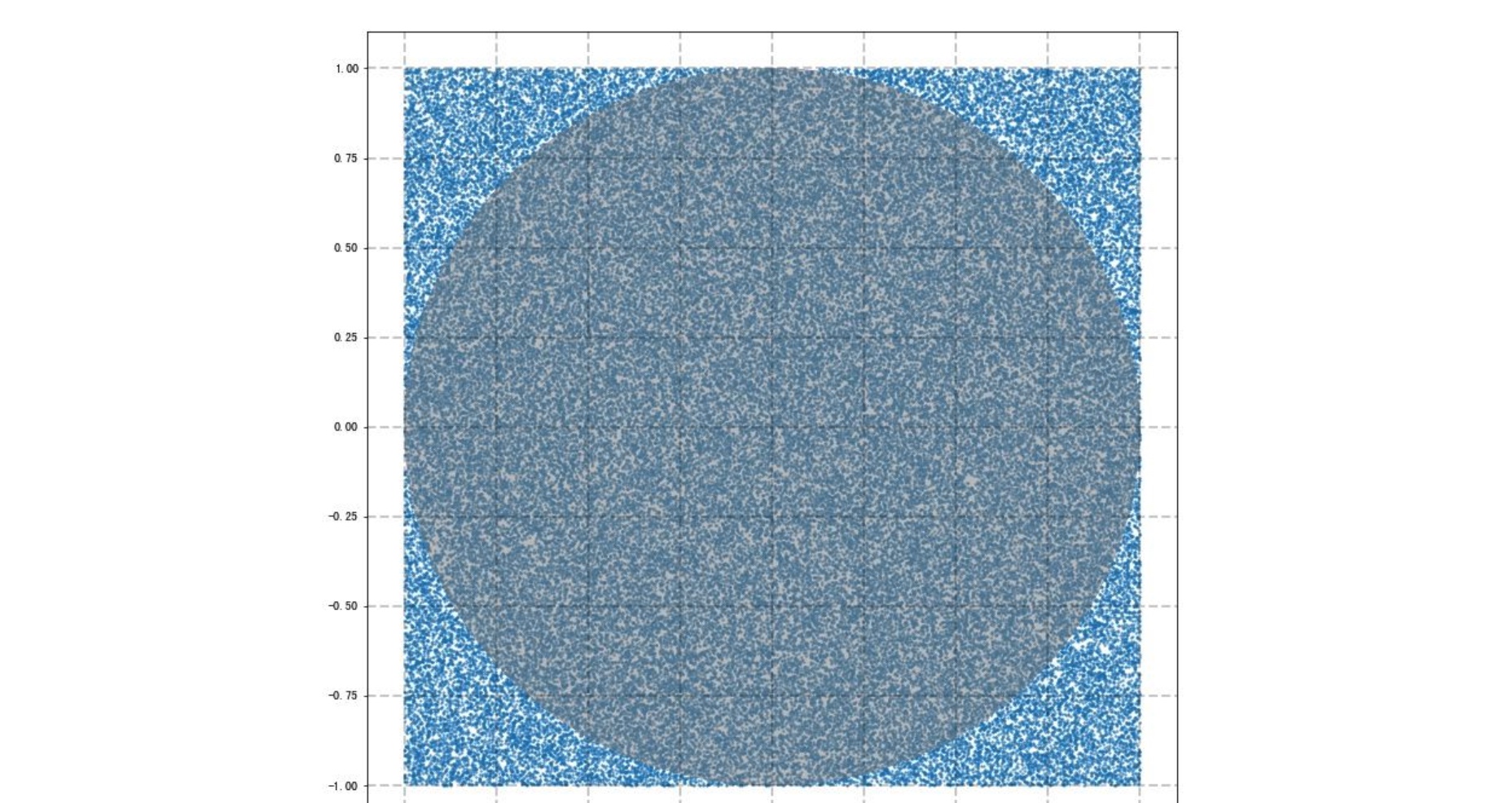
For example, consider a circle inscribed in a unit square. Given that the circle and the square have a ratio of areas that isπ/4, the value of π can be approximated using a Monte Carlo method:
- Draw a square, then inscribe a circle within it.
- Uniformly scatter objects of uniform size over the square.
- Count the number of objects inside the circle and the total number of objects.
- The ratio of the two counts is an estimate of the ratio of the two areas, which is π/4. Multiply the result by 4 to estimate π.
简单写法:
import random
from math import sqrt, pi

x = y = inn = out = 0.0

tolerance = 1e-5
piApproximation = 0.0
# for i in range(30000):
while abs(pi - piApproximation) > tolerance:
    x = random.random()
    y = random.random()
    # print(x, y)
    # print(sqrt(x * x + y * y))
    # 假设正方形边长为2.0
    # 点到圆心的距离需要小于1.0, 才证明点在圆内
    if sqrt(x**2 + y**2)<1.0:
    # if (x**2 + y**2) <= 1.0:
        inn += 1.0
    else:
        out += 1.0
    piApproximation = 4.0 * (inn / (inn+out))

print(inn)
print(out)
print(piApproximation)
# print(inn/30000 * 4)
print(inn / (out + inn) * 4)
π的求解
正方形的面积公式为 $S = a^2$,圆的面积公式为 $S =π * r^2$,可以用蒙特卡罗模拟,近似计算出π的近似值.
正方形内部有一个相切的圆,它们的面积之比是π/4 (因为π*r^2) / (2r)^2Å. 现在,在这个正方形内部,随机产生n个点,计算它们与中心点的距离,并且判断是否落在圆的内部。若这些点均匀分布,则圆周率 pi=4 * count/n, 其中count表示落到圆内投点数, n表示总的投点数
import numpy as np
import matplotlib.pyplot as plt
from matplotlib.patches import Circle

# 随机值数量 半径 圆心位置
# n = 100000
n = 10
r = 1.0
a,b, = 0.0, 0.0

np.random.seed(42)

y_max = b + r  # 1
y_min = b - r  # -1
x_max = a + r  # 1
x_min = a - r  # -1

# np.random.uniform()函数生成均匀分布的随机数
x = np.random.uniform(x_min,x_max,n) # [-0.25091976  0.90142861  0.46398788  0.19731697, ...
y = np.random.uniform(y_min,y_max,n) # [-0.95883101  0.9398197   0.66488528 -0.57532178, ....
print(x)
print('======')
print(y)
print('=======')
distance = np.sqrt((x-a)**2+(y-b)**2) # 点到圆心的距离
print(distance) # [0.99111939 1.30224215 0.81077567 0.608218, ...

count = sum(np.where(distance <= r,1,0))
print(count)

pai = 4 * count / n

print('π的值为:',pai)

fig = plt.figure(figsize = (12,12))
fig.add_subplot(1,1,1)
plt.scatter(x,y,marker='.',s = 10,alpha = 0.5)
yuan = fig.add_subplot(1,1,1)
circle = Circle(xy = (a,b),radius = r, alpha = 0.5 ,color = 'gray')
yuan.add_patch(circle)
plt.grid()
yuan.grid(color='k' ,linestyle='--', alpha = 0.2,linewidth=2) # 设置背景网格线的样式
# 绘制圆形
随机种子数在10000的时候,计算π值波动还比较大,将随机数量变为100000之后,π值比较接近了,重复多次后,可以取得更接近的实际的结果
C# code
using System;

class MainClass {
  public static void Main (string[] args) {
      // Construct a random number generator that generates random number greater than or equal to 0.0, and less than 1.0
      Random rand = new Random();

      // Approximate pi to within 5 digits.
      double tolerance = 1e-5;

      double piApproximation = 0;
      int total = 0;
      int numInCircle = 0;
      double x, y; // Coordinates of the random point.

      // Generate random points until our approximation within the desired tolerance.
      while ( Math.Abs( Math.PI - piApproximation ) > tolerance )
      {
        x = rand.NextDouble();
        y = rand.NextDouble();
        if ( x * x + y * y <= 1.0 ) // Is the point in the circle?
        {
          ++numInCircle;
        }
        ++total;
        piApproximation = 4.0 * ( (double) numInCircle / (double) total );
      }

      Console.WriteLine();

      Console.WriteLine( "Pi calculated to within {0} digits with {1} random points.",
        -Math.Log10( tolerance ), total );
      Console.WriteLine( "Approximated Pi = {0}", piApproximation );
  }
}
求定积分
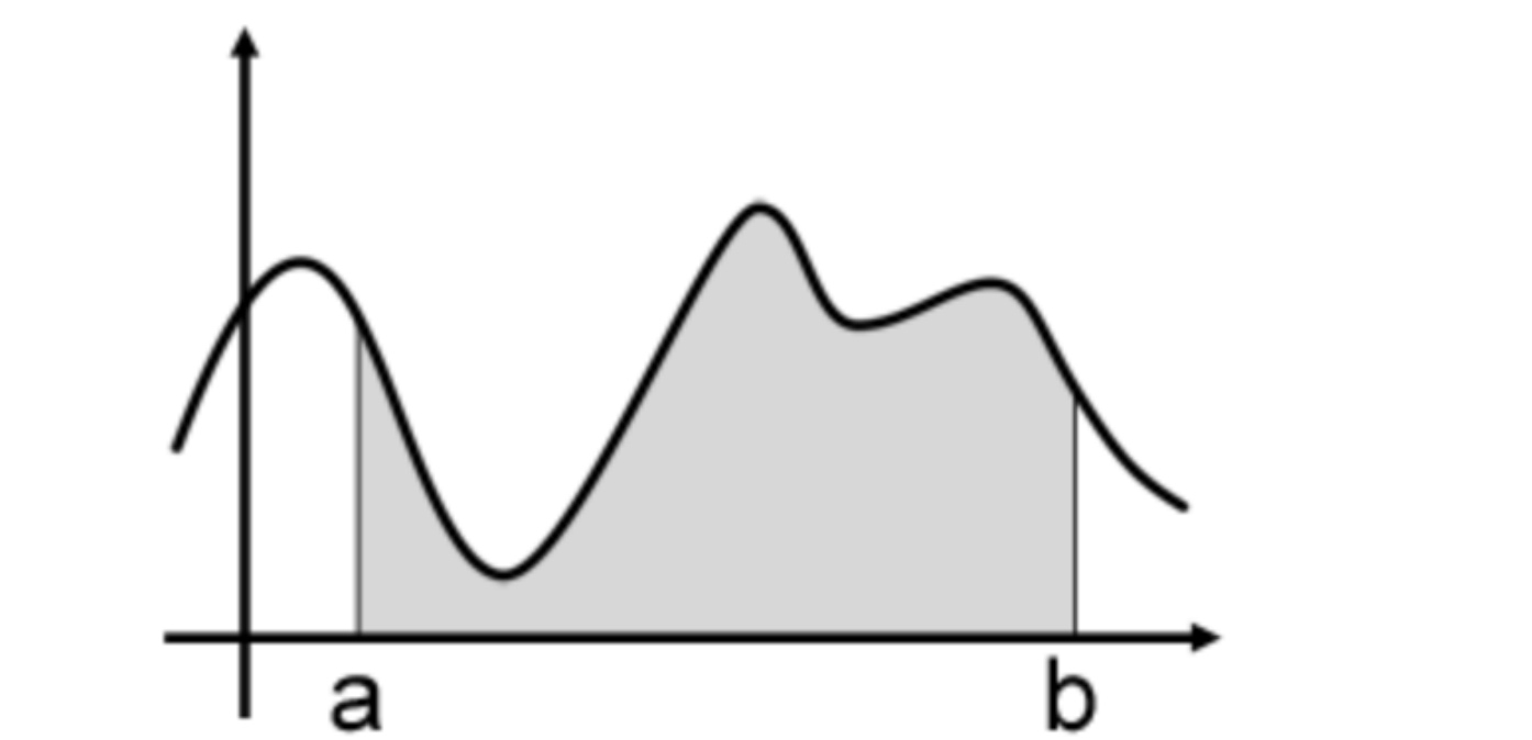 当在[a,b]之间随机取一点x时,它对应的函数值就是f(x).
然后可以用$f(x) * (b - a)$来粗略估计曲线下方的面积,也就是需要求的积分值,当然这种估计(或近似)是非常粗略的. 具体如下:
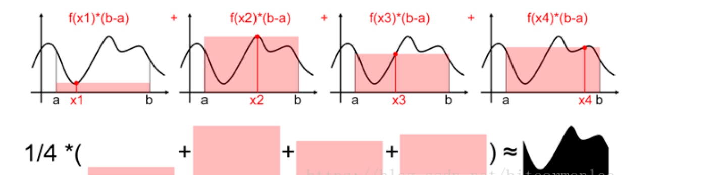
在此图中,做了四次随机采样,得到了四个随机样本$x1,x2,x3,x4$并且得到了这四个样本的$f(x_i)$的值分别为$f(x_1),f(x_2),f(x_3),f(x_4)$. 对于这四个样本,每个样本能求一个近似的面积值,大小为$f(xi)∗(b−a)$.
为什么能这么干么?对照图下面那部分很容易理解,每个样本都是对原函数f的近似,所以可以认为$f(x)$的值一直都等于$f(xi)$.
按照图中的提示,求出上述面积的数学期望,就完成了蒙特卡洛积分.
如果用数学公式表达上述过程:
$$\begin{aligned}
S & = \frac{1}{4}(f(x_1)(b-a) + f(x_2)(b-a) + f(x_3)(b-a) + f(x_4)(b-a)) \\
& = \frac{1}{4}(b-a)(f(x_1) + f(x_2) + f(x_3) + f(x_4)) \\
& = \frac{1}{4}(b-a) \sum_{i=1}^4 f(x_i)
\end{aligned}$$
通用情况
假设要计算的积分:
$$I = \int _a ^ b g(x) dx$$
其中被积函数$g(x)$在[a,b]内可积. 如果选择一个概率密度函数为$f_{X}(x)$的方式进行抽样,并且满足$\int _a ^ b f_X(x)dx = 1$,那么令$g^*(x) = \frac{g(x)}{f_X(x)}$,原有的积分可以写成如下形式:
$$I = \int _a ^ b g^*(x) f_X(x)dx$$
那么求积分的步骤应该是:
- 产生服从分布律FXFX的随机变量Xi(i=1,2,⋯,N)Xi(i=1,2,⋯,N)
- 计算均值
$$\overline I = \frac{1}{N} \sum_{i = 1}^N g^*(X_i)$$ 此时有 $$\overline I \approx I$$
在实际应用中,我们最常用的还是取$f_X$为均匀分布:
$$f_X(x) = \frac{1}{b - a}, a \le x \le b$$
此时
$$g^*(x) = (b-a)g(x)$$
代入积分表达式有:
$$I = (b-a) \int_a^b g(x) \frac{1}{b-a}dx$$
最后有
$$\overline I = \frac{b-a}{N}\sum_{i=1}^Ng(X_i)$$
代码
假设求$\int_0^1 x^2 dx$的值:
n = 100000
x_min, x_max = 0.0, 1.0
y_min, y_max = 0.0, 1.0

count = 0
for i in range(0, n):
    x = random.uniform(x_min, x_max)
    y = random.uniform(y_min, y_max)
    # x*x > y,表示该点位于曲线的下面。所求的积分值即为曲线下方的面积与正方形面积的比。
    if x*x > y:
        count += 1

integral_value = count / float(n)
print('定积分的结果为: ', integral_value)

fig = plt.figure(figsize = (12,12))
axes = fig.add_subplot(1,1,1)
axes.plot(x, y,'o',markersize = 1)
# 绘制散点图

xi = np.linspace(0,1,100)
yi = xi ** 2
plt.plot(xi,yi,'--r')
plt.fill_between(xi, yi, 0, color ='gray',alpha=0.5,label='area')
plt.grid()
# 绘制 y = x**2 面积图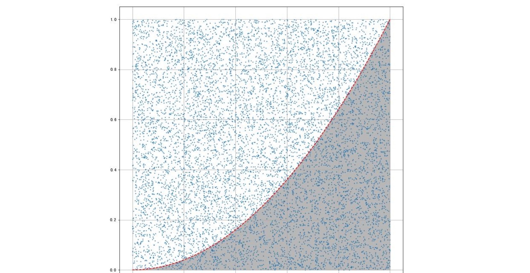
产品厚度
某产品由八个零件堆叠组成。也就是说,这八个零件的厚度总和,等于该产品的厚度。
已知该产品的厚度,必须控制在27mm以内,但是每个零件有一定的概率,厚度会超出误差。请问有多大的概率,产品的厚度会超出27mm?
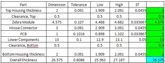
取100000个随机样本,每个样本有8个值,对应8个零件各自的厚度。计算发现,产品的合格率为99.9979%,即百万分之21的概率,厚度会超出27mm
证券市场
证券市场有时交易活跃,有时交易冷清。下面是你对市场的预测。
- 如果交易冷清,你会以平均价11元,卖出5万股。
- 如果交易活跃,你会以平均价8元,卖出10万股。
- 如果交易温和,你会以平均价10元,卖出7.5万股。
As a result, you expect to sell 75,000 units (i.e., (50,000+75,000+100,000)/3 = 75,000) at an average selling price of \$9.67 per unit (i.e., (\$11+\$10+\$8)/3 = $9.67)
calculates Net Profit based on average sales volume, average selling price, and average unit cost. Flawed Average = 75,000 * (\$9.67 - \$6.5) - 12,000 = 117,500 (The true average Net Profit is closer to $93,000, the average will nearly always be much less than \$117,750)
已知你的成本(unit cost)在每股5.5元到7.5元之间,平均是6.5元。请问接下来的交易,你的净利润会是多少?
取1000个随机样本,每个样本有两个数值:一个是证券的成本(5.5元到7.5元之间的均匀分布),另一个是当前市场状态(冷清、活跃、温和,各有三分之一可能
- 1000次抽样,每次按均匀分布随机选定一个成本值、同时按1/3的概率选中一个市场情境,然后拿这两个参数可计算出净利润、平均利润,千次加总并取均值就是结果。1000次抽样的技术本身就是蒙特卡罗模拟
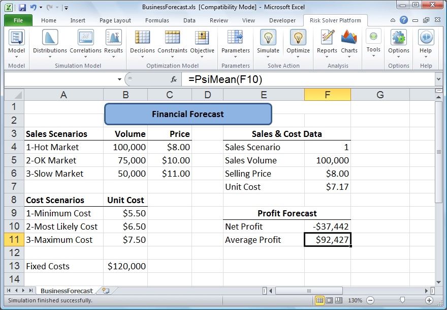
Net profit will be calculated as Net Profit = Sales Volume* (Selling Price - Unit cost) - Fixed costs. Fixed costs (for overhead, advertising, etc.) are known to be $120,000
模拟计算得到,平均净利润为92, 427美元
### way1
avg_cost = 6.5
sum_profit = 0
for i in range(1000):
    # cost = random.uniform(5.5,7.5)
    avg_sell = random.choice([(11,50000),(8,100000),(10,75000)])
    avg_profit = (avg_sell[0] - avg_cost) * avg_sell[1] - 120000  # 120000 is fixed costs
    sum_profit += avg_profit

avg_profit = sum_profit / 1000
print(avg_profit)  # 92775.0

### way2
net_profit = 0
for i in range(1000):
    cost = random.uniform(5.5,7.5)
    profit = (11 - cost)*50000 + (8 - cost)*100000 + (10 - cost)*75000 - 120000*3  # 120000 is fixed costs
    net_profit += profit
res = net_profit / (3*1000)
print(res)   # 92025.0
C#:
using System;

class MainClass {
  public static void Main (string[] args) {

      Random rand = new Random();
      double net_profit = 0.0;

      for(int i =0; i< 1000; i++){
        double cost = (rand.NextDouble() * 2.0) + 5.5;
        // Console.WriteLine(cost);
        double profit = (11 - cost)*50000 + (8 - cost)*100000 + (10 - cost)*75000 - 120000*3;

        net_profit += profit;

      }
      net_profit = net_profit / (3*1000);
      Console.WriteLine( "Net profit = {0}", net_profit );

  }
}
using System;

class MainClass {
  public static void Main (string[] args) {

      Random rand = new Random();
      double net_profit = 0.0;
      double avg_cost = 6.5;
      int[][] pos = new int[3][]{new int[]{11,50000}, new int[]{8,100000}, new int[]{10,75000}};

      // int temp = rand.Next(pos.Length);
      // Console.WriteLine(pos);
      // Console.WriteLine(pos.Length);
      // Console.WriteLine(temp);
      // Console.WriteLine(pos[temp][0]);

      for(int i =0; i< 1000; i++){
        int temp = rand.Next(pos.Length);
        double cost = pos[temp][0];
        double vol = pos[temp][1];
        double profit = (cost - avg_cost) * vol - 120000;

        net_profit += profit;

      }
      net_profit = net_profit / 1000;
      Console.WriteLine( "Net profit = {0}", net_profit );

  }
}
stock price prediction using monte carlo
- stock price data in dataframe
- calculate log return
- log_return = log(1 + data.pct_change())
- pct_change() stands for percentage change <==> moving average
- calculate mean, variance and std
- u = log_return.mean()
- var = log_return.var()
- stdev = log_return.std()
- compute the drift component (the best approximation of future rates of return of the stock)
$drift = u - \frac{1}{2} \cdot var $- average log return - half its variance
- Brownian motion
- first component:
$r = drift + stdev * e^r $- Brownian motion comprises the sum of the drift and standard deviation of adjusted by e to the power of r
- second component:
- a random variable Z: Z corresponds to the distance between the mean and the events, expressed as the number of standard deviations
- E.g. norm.ppf(0.95) = 1.65
- if an event has a 95% chance of occurring, the distance between this event and mean will approximately 1.65 standard deviations
- Z = spicy.stat.norm.ppf(np.random.rand(10,2))
- use the probabilities generated by the rand and convert them into distances from the mean zero as measured by the number of standard deviations
$daily_returns = e^r$$ r = drift + stdev * z $- e is Euler’s number / natural number
- Next Day’s Price = Today’s Price x e^(Drift+Random Value)
- time_interval is 1000 (since it is forecasting the stock price for the upcoming 1000days)
- iteration is 10 (ask computer to produce 10 series of future stock price prediction)
- daily_returns = np.exp(drift + stdev * norm.ppf(np.random.rand(time_interval, iteration)))
- 1000rows x 10cols
- S0 = data.iloc[-1] which is the last adjusted closing price of the stock
- price_list= np.zeros_like(daily_returns) – create a price_list, the same dimension as the daily_returns matrix with all 0.0
- price_list[0] = S0 - Set the values on the first row of the price_list array equal to S0
- Create a loop in the range (1 to t_intervals) that reassigns to the price in time t the product of the price in day (t-1) with the value of the daily returns in t
- for t in range(1, t_intervals): price_list[t] = price_list[t – 1] * daily_returns[t]
- first component:
code:
#Import Libraries
import numpy as np
import pandas as pd
import pandas_datareader as wb
import matplotlib.pyplot as plt
from scipy.stats import norm
%matplotlib inline

#Settings for Monte Carlo asset data, how long, and how many forecasts
ticker = 'XTZ_USD' # ticker
t_intervals = 30 # time steps forecasted into future
iterations = 25 # amount of simulations
#Acquiring data
data = pd.read_csv('XTZ_USD Huobi Historical Data.csv',index_col=0,usecols=['Date', 'Price'])
data = data.rename(columns={"Price": ticker})
#Preparing log returns from data
log_returns = np.log(1 + data.pct_change())
#Plot of asset historical closing price
data.plot(figsize=(10, 6));

#Plot of log returns
log_returns.plot(figsize = (10, 6))

#Setting up drift and random component in relation to asset data
u = log_returns.mean()
var = log_returns.var()
drift = u - (0.5 * var)
stdev = log_returns.std()
daily_returns = np.exp(drift.values + stdev.values * norm.ppf(np.random.rand(t_intervals, iterations)))
#Takes last data point as startpoint point for simulation
S0 = data.iloc[-1]
price_list = np.zeros_like(daily_returns)
price_list[0] = S0
#Applies Monte Carlo simulation in asset
for t in range(1, t_intervals):
    price_list[t] = price_list[t - 1] * daily_returns[t]

#Plot simulations
plt.figure(figsize=(10,6))
plt.plot(price_list);
简单版公式: $前一天的价格 * e^{random_return * randomNum(1-Noofday)}$
Ref
- https://blog.csdn.net/bitcarmanlee/article/details/82716641
- https://zhuanlan.zhihu.com/p/41755547
- http://www.ruanyifeng.com/blog/2015/07/monte-carlo-method.html
- https://www.solver.com/monte-carlo-simulation-example
- https://datascienceplus.com/how-to-apply-monte-carlo-simulation-to-forecast-stock-prices-using-python/
- https://medium.com/fintechexplained/monte-carlo-simulation-engine-in-python-a1fa5043c613
- https://towardsdatascience.com/python-risk-management-monte-carlo-simulations-7d41c891cb5
https://www.shuzhiduo.com/A/VGzlbNGV5b/
https://www.shuzhiduo.com/A/x9J2QZ1Vz6/
马尔可夫链蒙特卡洛采样 (Markov Chain Monte Carlo - MCMC)
MCMC 方法用于通过在概率空间中进行随机采样以近似地得出某一感兴趣参数的后验分布
https://baijiahao.baidu.com/s?id=1628127197886312445&wfr=spider&for=pc
https://baijiahao.baidu.com/s?id=1588750123445231830&wfr=spider&for=pc