4. Sequences, Time Series and Prediction

2019-11-18 19 minutes read

Keras

#DL • #Keras • #Andrew

views 3850 words

Sequences and Prediction

Time series is typically defined as an ordered sequence of values that are usually equally spaced over time. For example, every year in my Moore’s law charts or every day in the weather forecast. In each of these examples, there is a single value at each time step(univariate time series chart). Multiple values at each time steps call Multivariate time series.

Application in Machine Learning:

Prediction of forecasting based on the data
Imputation (to project back into the past to see how to got to current trend)
Fill in holes for non-exist data with imputation
detect anomalies
spot patterns in time series data that determine what generated the series itself (E.g. analyze sound waves to spot words in them)

Common Pattern:

trend
seasonality
combination of both trend and seasonality
set of random values (unpredictable and produce white noise)
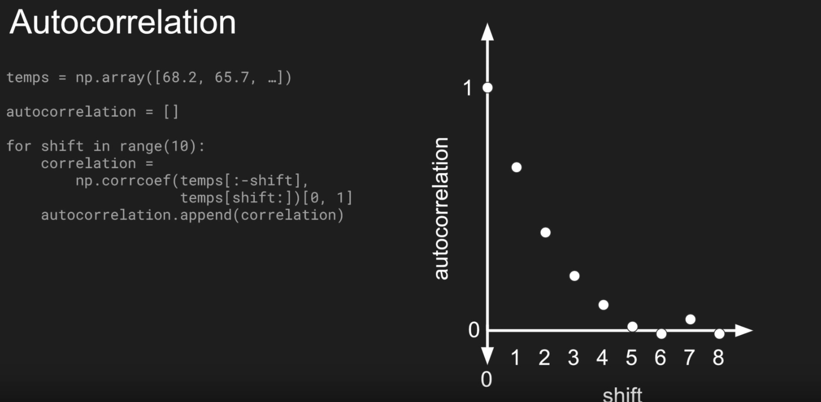
auto correlated time series
- $v(t) = 0.99 \times v(t-1) + occasional \; spike$
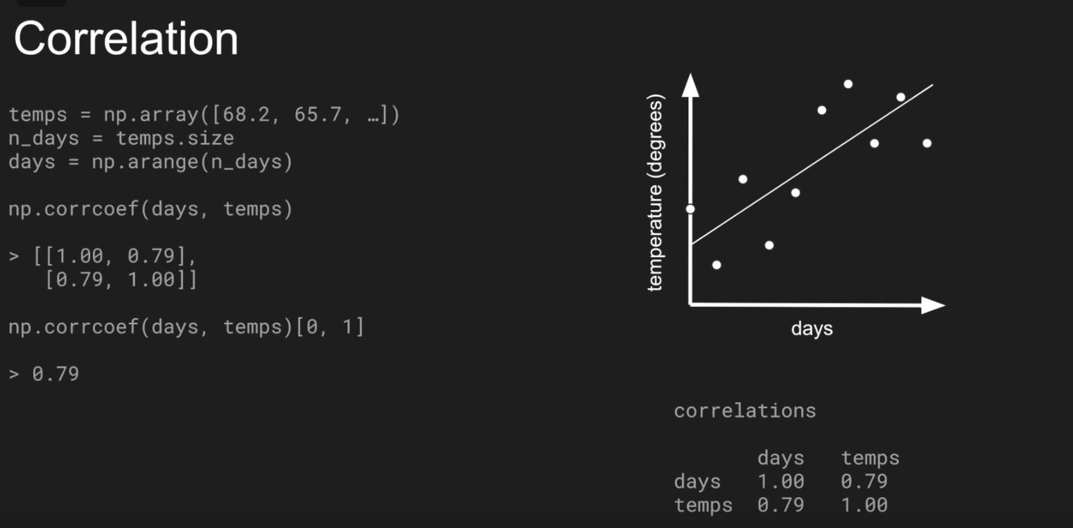
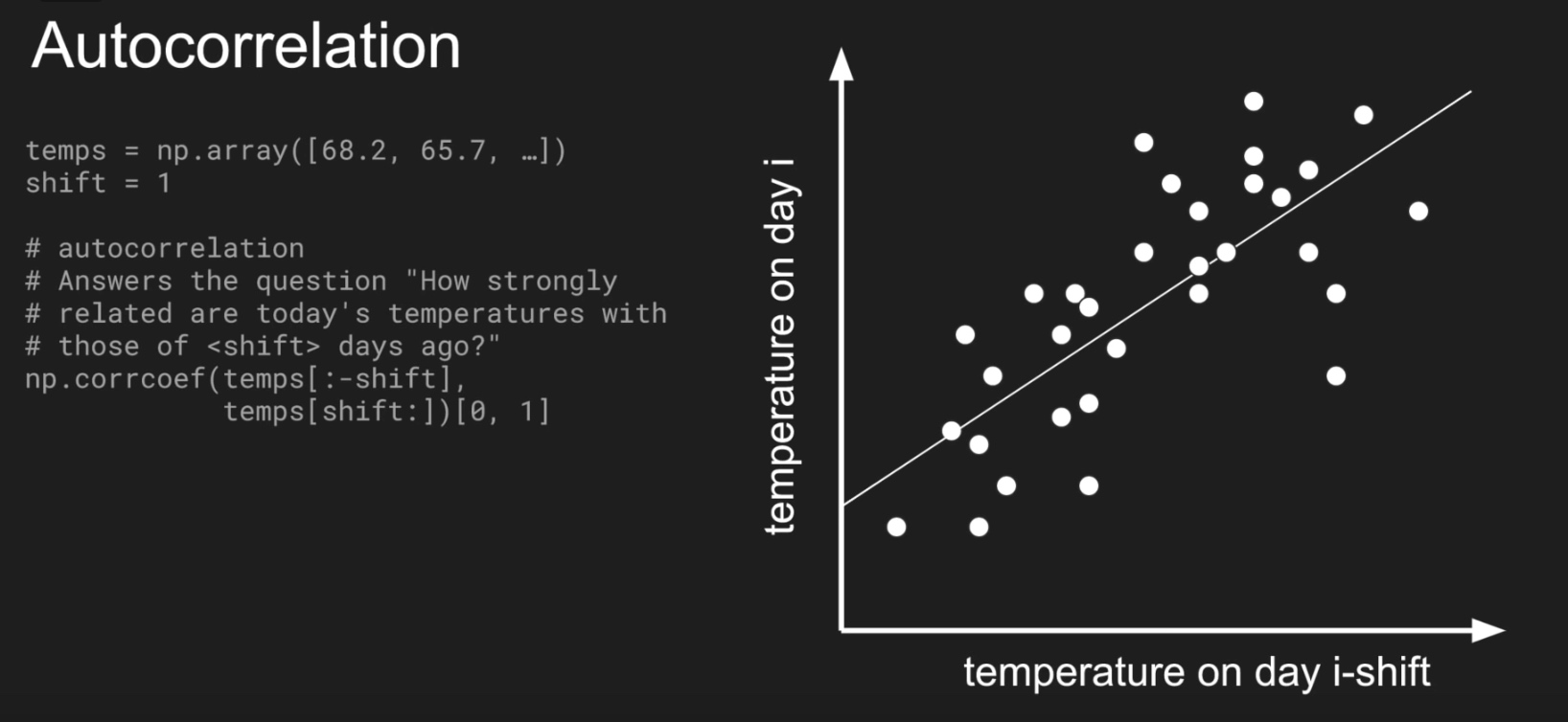
- it correlates with a delayed copy of itself, often called a lag
- Autocorrelation measures the relationship between a variable’s current value and its past values.

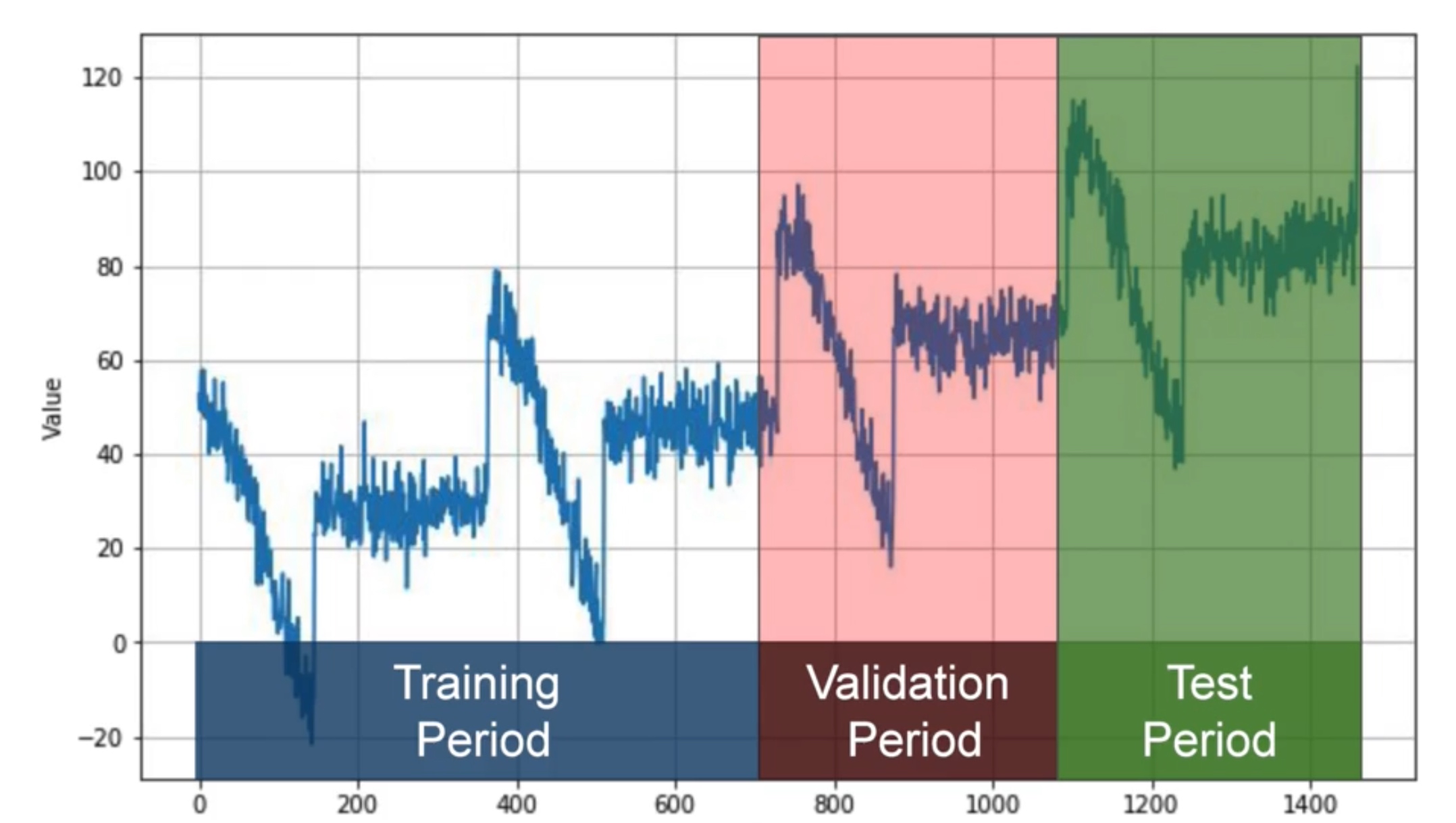
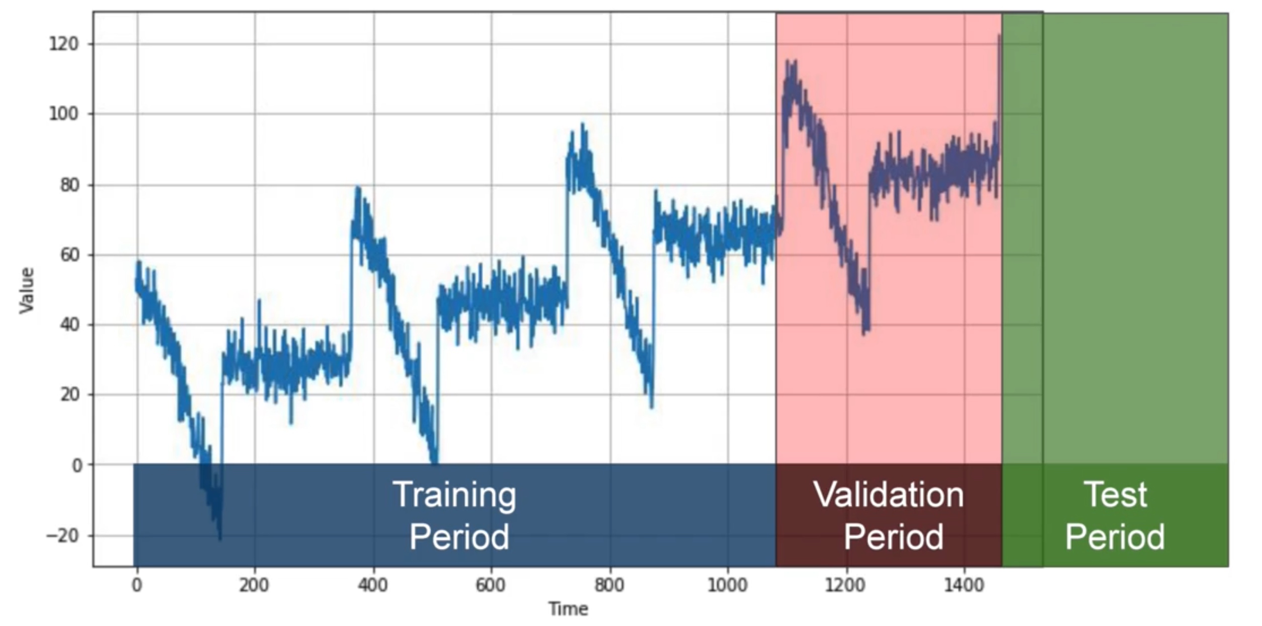
Split time series:

Fixed Partitioning: -w1078 -w1254

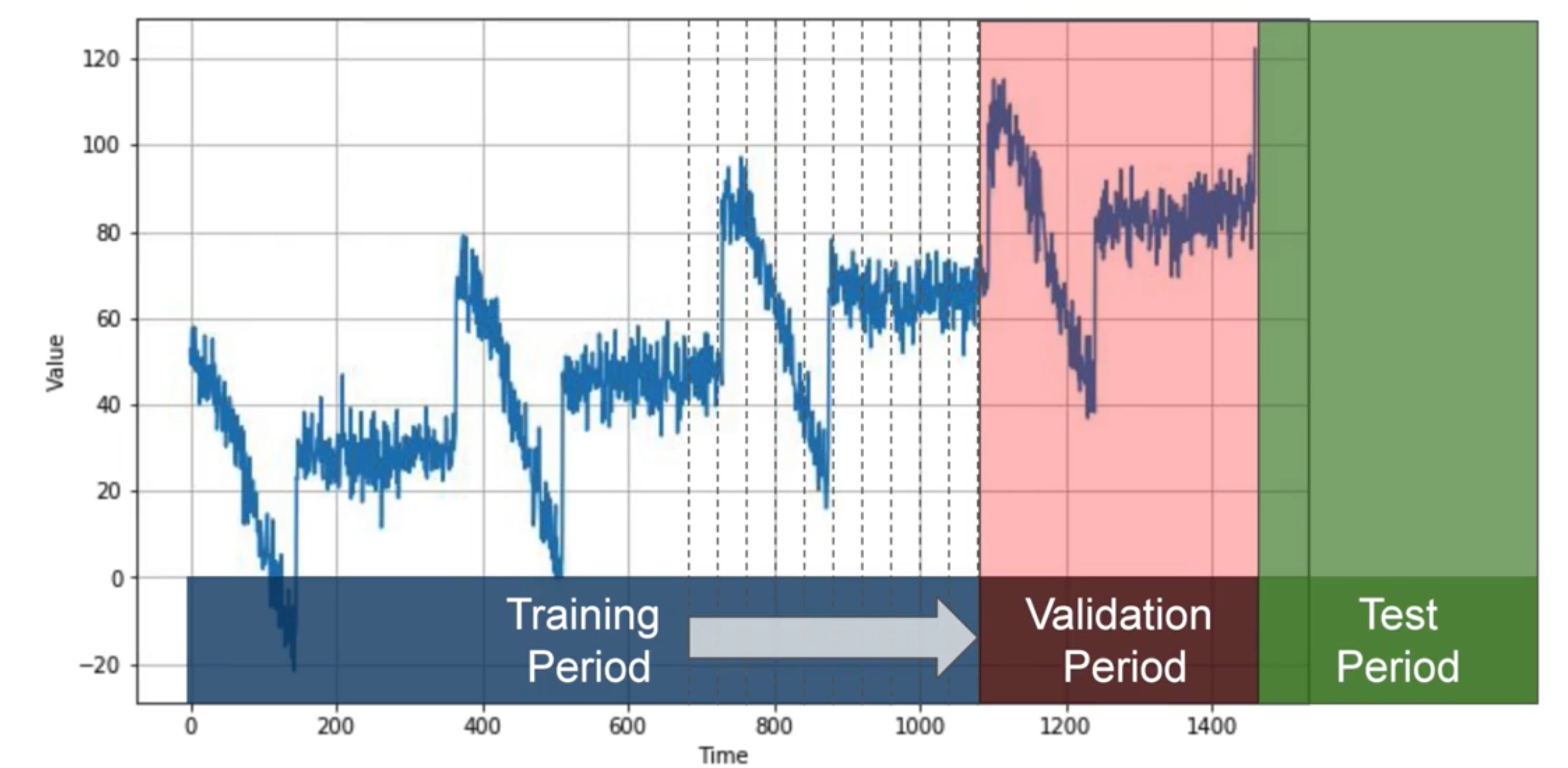
Roll-Forward Partitioning

start with a short training period, and gradually increase it, say by one day at a time, or by one week at a time. At each iteration, train the model on a training period. And use it to forecast the following day, or the following week, in the validation period.

Metrics of evaluation of model:

errors = forecasts - actual
mean square error: mse = np.square(errors).mean()
- square is to get rid of negative value
root mean square error: rmse = np.sqrt(mse)
- calculation to be of the same scale as the original errors
mean absolute error: mae = np.abs(errors).mean()
- use abs() to get rid of negative value and not penalize large errors as much as mse does
- tf.keras.metrics.mean_absolute_error(x_valid,naive_forecast).numpy()
mean absolute percentage error: mape = np.abs(errors / x_valid).mean()

Moving average - forcasting method -w1166

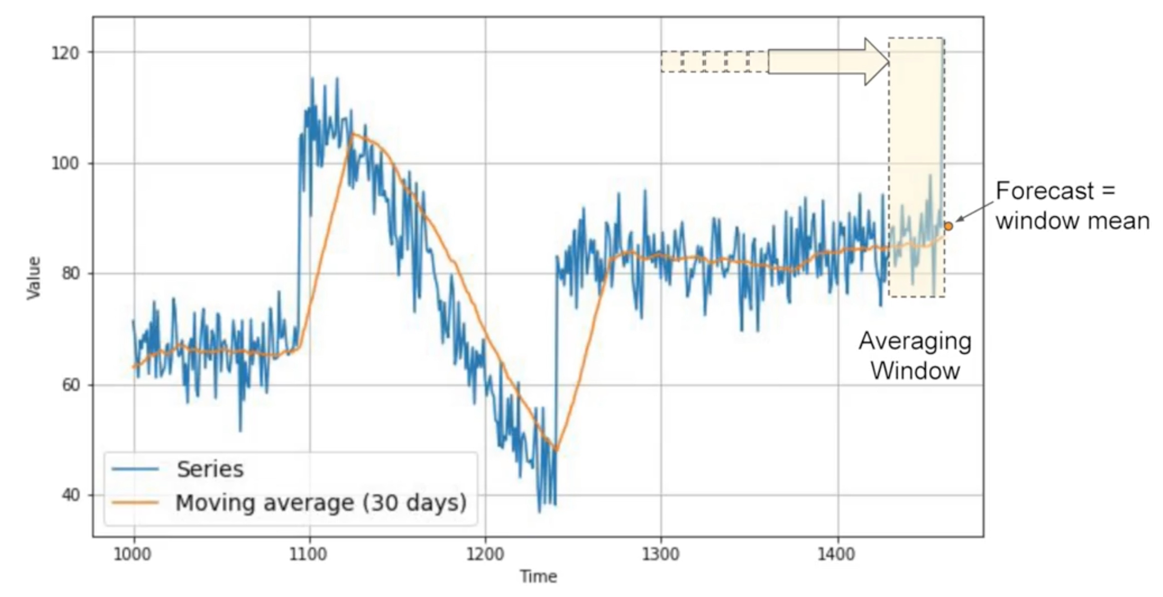
yellow line - plot of average
blue line - averaging window

Differencing - remove the trend and seasonality:

Instead of studying the time series itself, we study the difference between the value at time t and the value at a earlier period
- 365 as a period: Series(t) - Series(t-365)

Code:

This code block will set up the time series with seasonality, trend and a bit of noise.

import numpy as np
import matplotlib.pyplot as plt
import tensorflow as tf
from tensorflow import keras

def plot_series(time, series, format="-", start=0, end=None):
    plt.plot(time[start:end], series[start:end], format)
    plt.xlabel("Time")
    plt.ylabel("Value")
    plt.grid(True)

def trend(time, slope=0):
    return slope * time

def seasonal_pattern(season_time):
    """Just an arbitrary pattern, you can change it if you wish"""
    return np.where(season_time < 0.4,
                    np.cos(season_time * 2 * np.pi),
                    1 / np.exp(3 * season_time))

def seasonality(time, period, amplitude=1, phase=0):
    """Repeats the same pattern at each period"""
    season_time = ((time + phase) % period) / period
    return amplitude * seasonal_pattern(season_time)

def noise(time, noise_level=1, seed=None):
    rnd = np.random.RandomState(seed)
    return rnd.randn(len(time)) * noise_level

time = np.arange(4 * 365 + 1, dtype="float32")
baseline = 10
series = trend(time, 0.1)  
baseline = 10
amplitude = 40
slope = 0.05
noise_level = 5

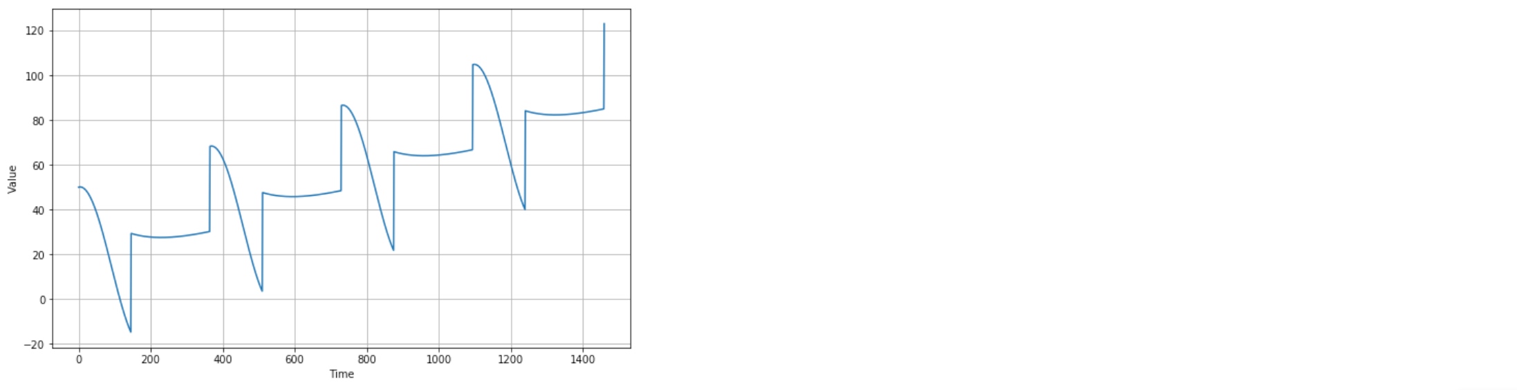
# Create the series
series = baseline + trend(time, slope) + seasonality(time, period=365, amplitude=amplitude)
# Update with noise
series += noise(time, noise_level, seed=42)

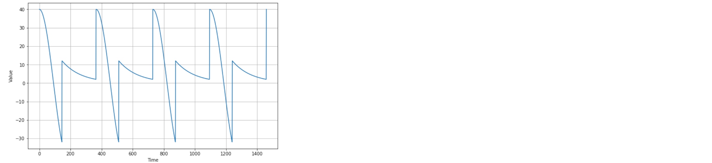
plt.figure(figsize=(10, 6))
plot_series(time, series)
plt.show()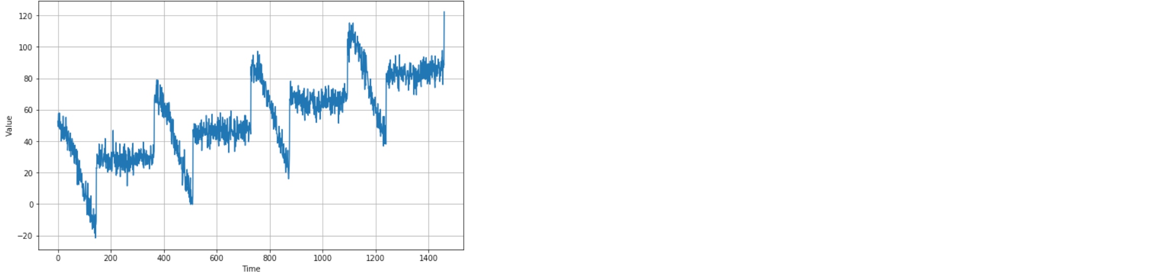

-w1140

Split the time series so can start forecasting

split_time = 1000
time_train = time[:split_time]
x_train = series[:split_time]
time_valid = time[split_time:]
x_valid = series[split_time:]
plt.figure(figsize=(10, 6))
plot_series(time_train, x_train)
plt.show()

plt.figure(figsize=(10, 6))
plot_series(time_valid, x_valid)
plt.show()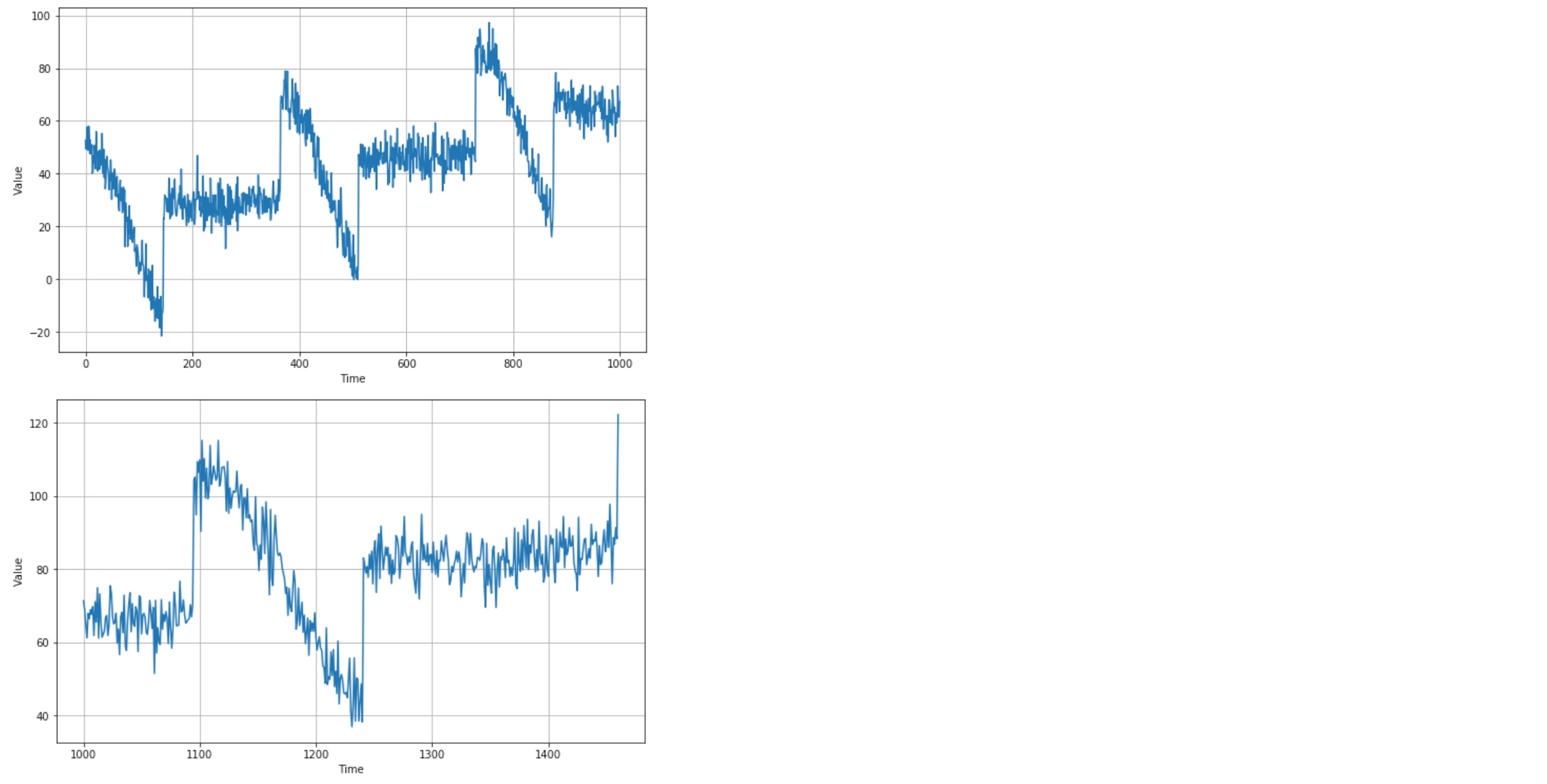

-w1101

Naive forecasting

Take the last value and assume that the next value will be the same one

naive_forecast = series[split_time - 1:-1]

plt.figure(figsize=(10, 6))
plot_series(time_valid, x_valid)
plot_series(time_valid, naive_forecast)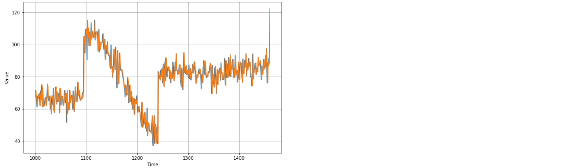

-w943

zoom in:

plt.figure(figsize=(10, 6))
plot_series(time_valid, x_valid, start=0, end=150)
plot_series(time_valid, naive_forecast, start=1, end=151)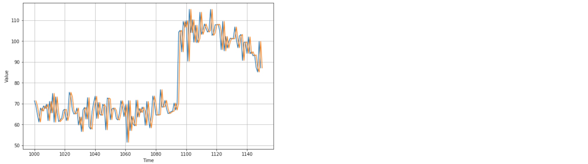

-w982 The naive forecast lags 1 step behind the time series.

Compute the mean squared error and the mean absolute error between the forecasts and the predictions in the validation period:

print(keras.metrics.mean_squared_error(x_valid, naive_forecast).numpy())
print(keras.metrics.mean_absolute_error(x_valid, naive_forecast).numpy())

# 61.827538
# 5.9379086

Moving Average forecasting

def moving_average_forecast(series, window_size):
  """Forecasts the mean of the last few values.
     If window_size=1, then this is equivalent to naive forecast"""
  forecast = []
  for time in range(len(series) - window_size):
    forecast.append(series[time:time + window_size].mean())
  return np.array(forecast)


moving_avg = moving_average_forecast(series, 30)[split_time - 30:]

plt.figure(figsize=(10, 6))
plot_series(time_valid, x_valid)
plot_series(time_valid, moving_avg)

print(keras.metrics.mean_squared_error(x_valid, moving_avg).numpy())
print(keras.metrics.mean_absolute_error(x_valid, moving_avg).numpy())

# 106.674576
# 7.142419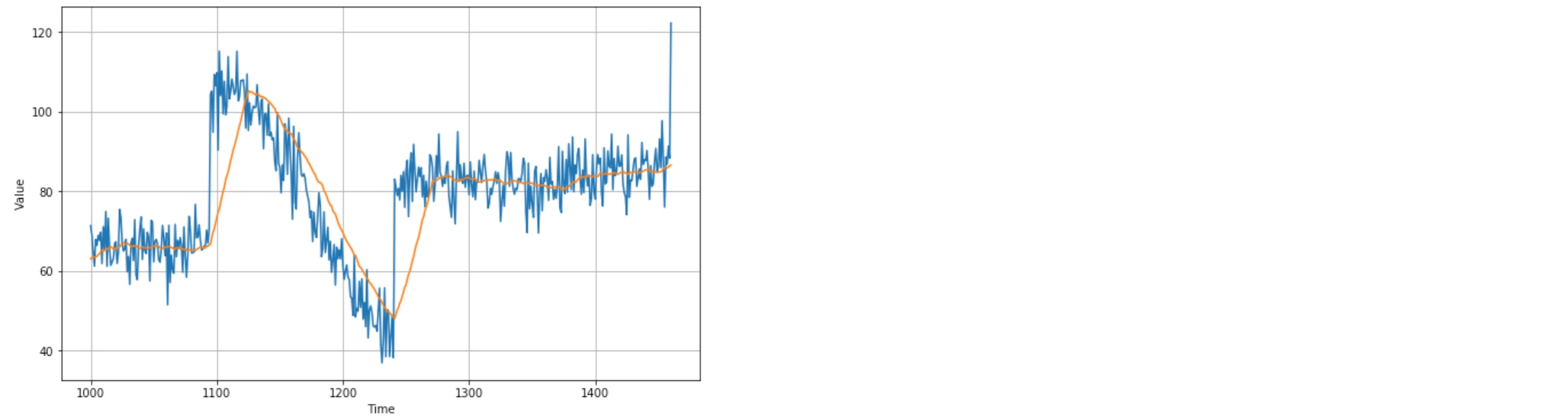

-w1028 That’s worse than naive forecast. The moving average does not anticipate trend or seasonality. So remove them by using differencing. Since the seasonality period is 365 days, we will subtract the value at time t – 365 from the value at time t.

diff_series = (series[365:] - series[:-365])
diff_time = time[365:]

plt.figure(figsize=(10, 6))
plot_series(diff_time, diff_series)
plt.show()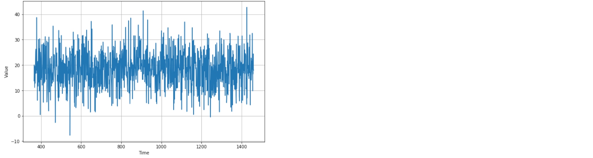

-w1026 The trend and seasonality are gone, so now can use the moving average:

diff_moving_avg = moving_average_forecast(diff_series, 50)[split_time - 365 - 50:]

plt.figure(figsize=(10, 6))
plot_series(time_valid, diff_series[split_time - 365:])
plot_series(time_valid, diff_moving_avg)
plt.show()
print(diff_moving_avg,len(diff_moving_avg)) # 461
print(series[split_time - 365:-365],len(series[split_time - 365:-365])) # 461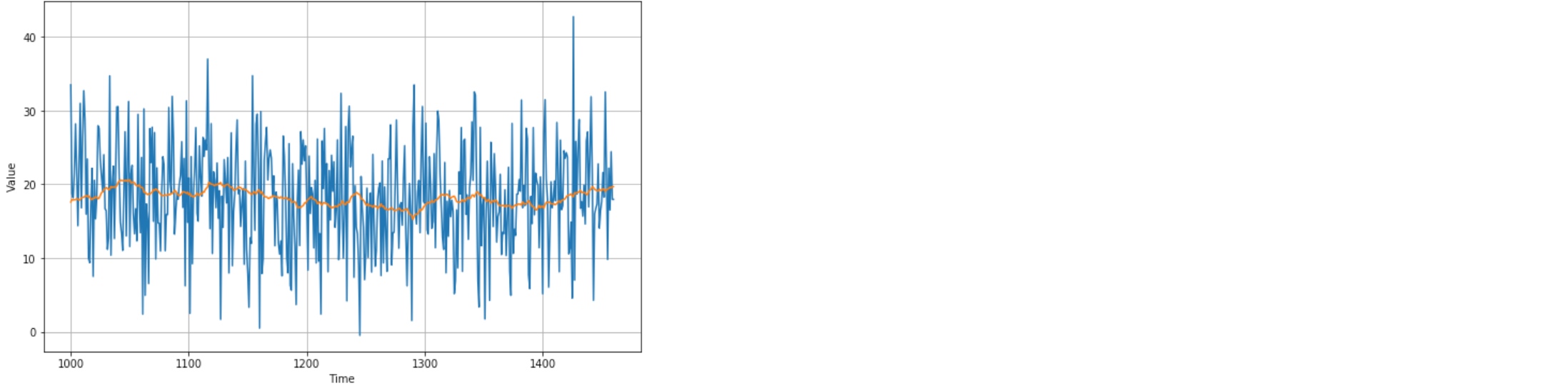

-w1098

Bring back the trend and seasonality by adding the past values from t – 365:

diff_moving_avg_plus_past = series[split_time - 365:-365] + diff_moving_avg

plt.figure(figsize=(10, 6))
plot_series(time_valid, x_valid)
plot_series(time_valid, diff_moving_avg_plus_past)
plt.show()


print(keras.metrics.mean_squared_error(x_valid, diff_moving_avg_plus_past).numpy())
print(keras.metrics.mean_absolute_error(x_valid, diff_moving_avg_plus_past).numpy())

# 52.973656
# 5.8393106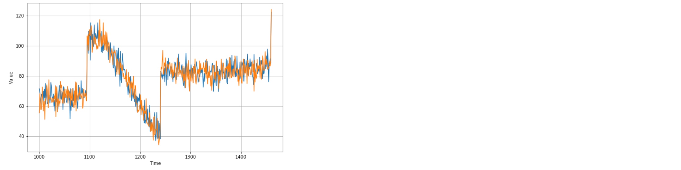

-w1117

Better than naive forecast. However the forecasts look a bit too random (noise), because we’re just adding past values, which were noisy.

So use a moving averaging on past values to remove some of the noise:

diff_moving_avg_plus_smooth_past = moving_average_forecast(series[split_time - 370:-360], 10) + diff_moving_avg

plt.figure(figsize=(10, 6))
plot_series(time_valid, x_valid)
plot_series(time_valid, diff_moving_avg_plus_smooth_past)
plt.show()

print(keras.metrics.mean_squared_error(x_valid, diff_moving_avg_plus_smooth_past).numpy())
print(keras.metrics.mean_absolute_error(x_valid, diff_moving_avg_plus_smooth_past).numpy())

# 33.45226
# 4.569442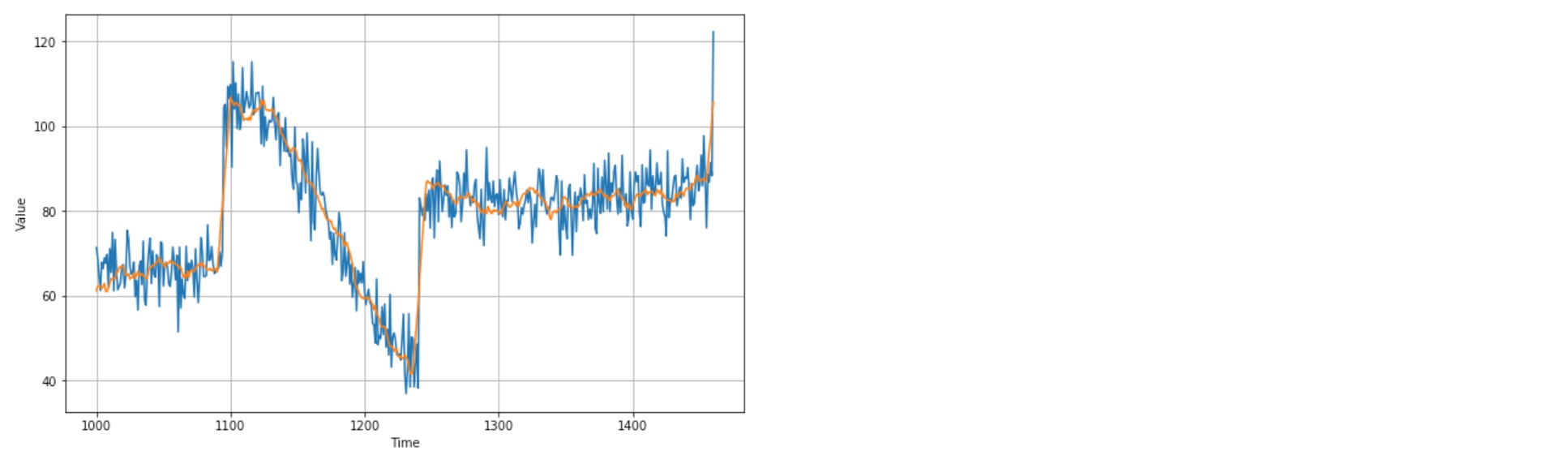

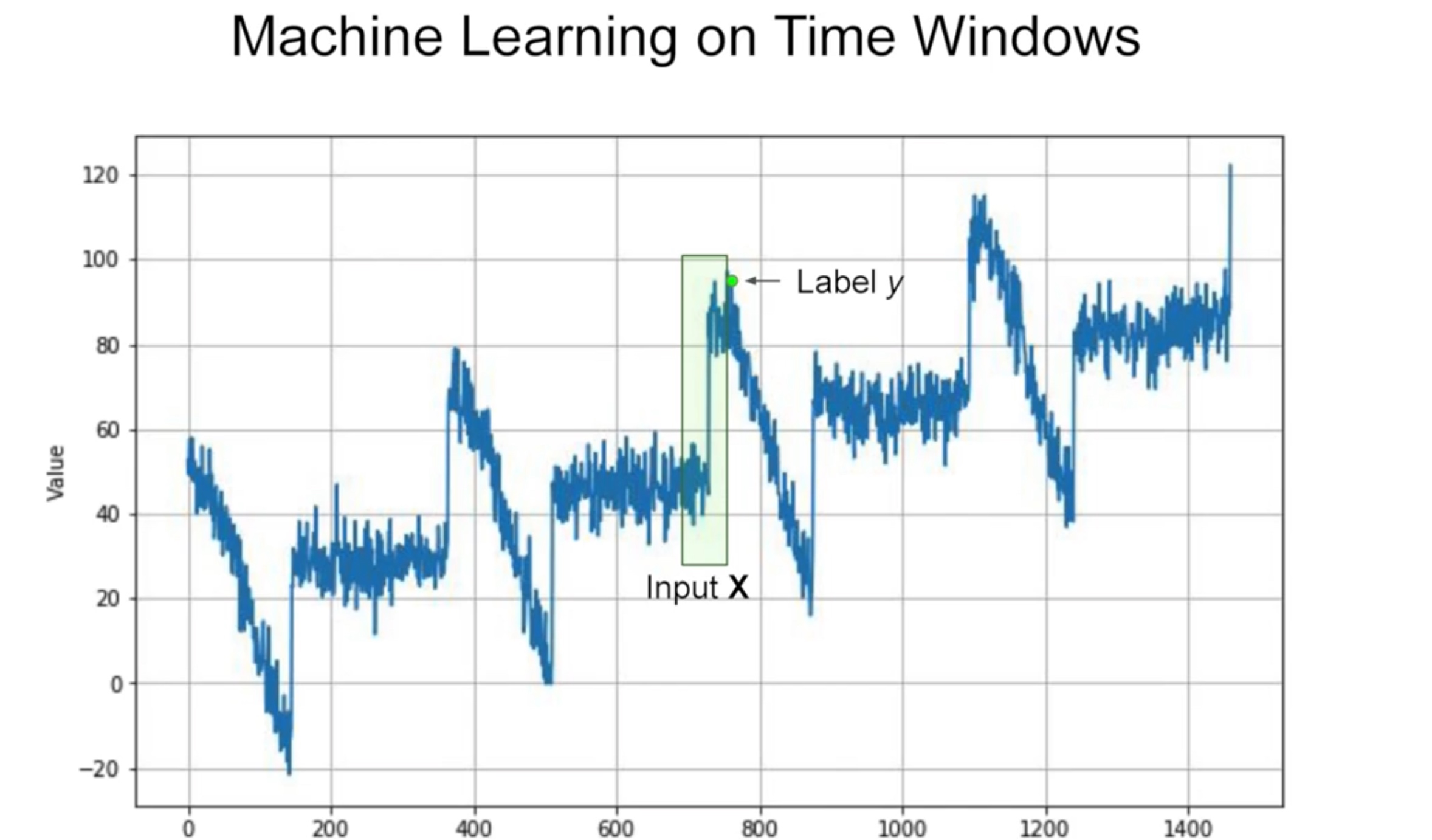
-w967

DNN for Time Series

Divide data into features and labels (Split a data series into windows) -w1178

dataset = tf.data.Dataset.range(10)
for val in dataset:
   print(val.numpy())

# 0
# 1
# 2
# 3
# 4
# 5
# 6
# 7
# 8
# 9

dataset = tf.data.Dataset.range(10)
dataset = dataset.window(5, shift=1)
for window_dataset in dataset:
  for val in window_dataset:
    print(val.numpy(), end=" ")
  print()

# 0 1 2 3 4 
# 1 2 3 4 5 
# 2 3 4 5 6 
# 3 4 5 6 7 
# 4 5 6 7 8 
# 5 6 7 8 9 
# 6 7 8 9 
# 7 8 9 
# 8 9 
# 9

dataset = tf.data.Dataset.range(10)
dataset = dataset.window(5, shift=1, drop_remainder=True) # truncate the data by dropping all of the remainders
for window_dataset in dataset:
  for val in window_dataset:
    print(val.numpy(), end=" ")
  print()

# 0 1 2 3 4 
# 1 2 3 4 5 
# 2 3 4 5 6 
# 3 4 5 6 7 
# 4 5 6 7 8 
# 5 6 7 8 9

dataset = tf.data.Dataset.range(10)
dataset = dataset.window(5, shift=1, drop_remainder=True) 
dataset = dataset.flat_map(lambda window: window.batch(5))
for window in dataset:
  print(window.numpy())

# [0 1 2 3 4]
# [1 2 3 4 5]
# [2 3 4 5 6]
# [3 4 5 6 7]
# [4 5 6 7 8]
# [5 6 7 8 9]

dataset = tf.data.Dataset.range(10)
dataset = dataset.window(5, shift=1, drop_remainder=True)
dataset = dataset.flat_map(lambda window: window.batch(5))
dataset = dataset.map(lambda window: (window[:-1], window[-1:]))
for x,y in dataset:
  print(x.numpy(), y.numpy())

# [0 1 2 3] [4]
# [1 2 3 4] [5]
# [2 3 4 5] [6]
# [3 4 5 6] [7]
# [4 5 6 7] [8]
# [5 6 7 8] [9]

dataset = tf.data.Dataset.range(10)
dataset = dataset.window(5, shift=1, drop_remainder=True)
dataset = dataset.flat_map(lambda window: window.batch(5))
dataset = dataset.map(lambda window: (window[:-1], window[-1:]))
dataset = dataset.shuffle(buffer_size=10)
for x,y in dataset:
  print(x.numpy(), y.numpy())

# [1 2 3 4] [5]
# [4 5 6 7] [8]
# [2 3 4 5] [6]
# [0 1 2 3] [4]
# [5 6 7 8] [9]
# [3 4 5 6] [7]

dataset = tf.data.Dataset.range(10)
dataset = dataset.window(5, shift=1, drop_remainder=True)
dataset = dataset.flat_map(lambda window: window.batch(5))
dataset = dataset.map(lambda window: (window[:-1], window[-1:]))
dataset = dataset.shuffle(buffer_size=10)
dataset = dataset.batch(2).prefetch(1)
for x,y in dataset:
  print("x = ", x.numpy())
  print("y = ", y.numpy())

# x =  [[5 6 7 8], [3 4 5 6]]
# y =  [[9], [7]]
# x =  [[0 1 2 3], [1 2 3 4]]
# y =  [[4], [5]]
# x =  [[2 3 4 5], [4 5 6 7]]
# y =  [[6], [8]]

Machine Learning on Time Windows

%tensorflow_version 2.x

import tensorflow as tf
import numpy as np
import matplotlib.pyplot as plt
print(tf.__version__)

def plot_series(time, series, format="-", start=0, end=None):
    plt.plot(time[start:end], series[start:end], format)
    plt.xlabel("Time")
    plt.ylabel("Value")
    plt.grid(True)

def trend(time, slope=0):
    return slope * time

def seasonal_pattern(season_time):
    """Just an arbitrary pattern, you can change it if you wish"""
    return np.where(season_time < 0.4,
                    np.cos(season_time * 2 * np.pi),
                    1 / np.exp(3 * season_time))

def seasonality(time, period, amplitude=1, phase=0):
    """Repeats the same pattern at each period"""
    season_time = ((time + phase) % period) / period
    return amplitude * seasonal_pattern(season_time)

def noise(time, noise_level=1, seed=None):
    rnd = np.random.RandomState(seed)
    return rnd.randn(len(time)) * noise_level

time = np.arange(4 * 365 + 1, dtype="float32")
baseline = 10
series = trend(time, 0.1)  
baseline = 10
amplitude = 40
slope = 0.05
noise_level = 5

# Create the series
series = baseline + trend(time, slope) + seasonality(time, period=365, amplitude=amplitude)
# Update with noise
series += noise(time, noise_level, seed=42)

split_time = 1000
time_train = time[:split_time]
x_train = series[:split_time]
time_valid = time[split_time:]
x_valid = series[split_time:]

window_size = 20
batch_size = 32
shuffle_buffer_size = 1000

def windowed_dataset(series, window_size, batch_size, shuffle_buffer):
  dataset = tf.data.Dataset.from_tensor_slices(series)
  dataset = dataset.window(window_size + 1, shift=1, drop_remainder=True)
  dataset = dataset.flat_map(lambda window: window.batch(window_size + 1))
  dataset = dataset.shuffle(shuffle_buffer).map(lambda window: (window[:-1], window[-1]))  # e.g. buffer size 1000, it will fill the buffer with first 1000 elements, pick one of them at random
  dataset = dataset.batch(batch_size).prefetch(1)
  return dataset

dataset = windowed_dataset(x_train, window_size, batch_size, shuffle_buffer_size)
print(dataset)
l0 = tf.keras.layers.Dense(1, input_shape=[window_size])
model = tf.keras.models.Sequential([l0])

model.summary()

model.compile(loss="mse", optimizer=tf.keras.optimizers.SGD(lr=1e-6, momentum=0.9))
model.fit(dataset,epochs=100,verbose=0)

print("Layer weights {}".format(l0.get_weights()))  # first array is W0, W1, ...., W19, second array is b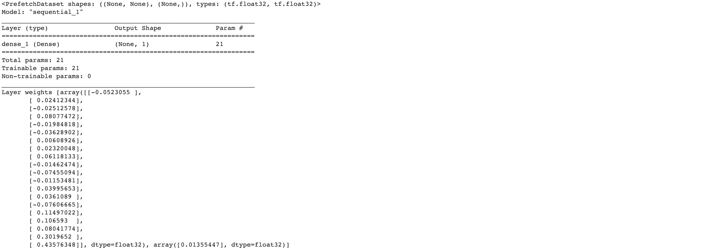

-w1135

print(series[1:21])
print(model.predict(series[1:21][np.newaxis]))

# [49.35275  53.314735 57.711823 48.934444 48.931244 57.982895 53.897125
#  47.67393  52.68371  47.591717 47.506374 50.959415 40.086178 40.919415
#  46.612473 44.228207 50.720642 44.454983 41.76799  55.980938]
# [[48.584476]]

forecast = []

for time in range(len(series) - window_size):
  forecast.append(model.predict(series[time:time + window_size][np.newaxis]))

forecast = forecast[split_time-window_size:]
results = np.array(forecast)[:, 0, 0]


plt.figure(figsize=(10, 6))

plot_series(time_valid, x_valid)
plot_series(time_valid, results)

tf.keras.metrics.mean_absolute_error(x_valid, results).numpy()
# 5.3161087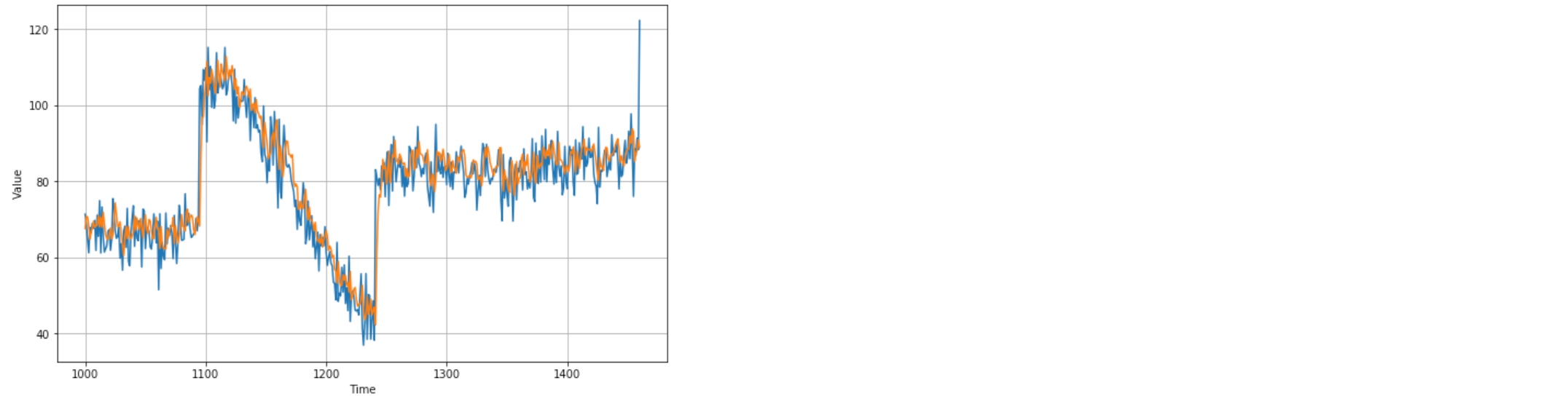

-w1076

DNN training

dataset = windowed_dataset(x_train, window_size, batch_size, shuffle_buffer_size)


model = tf.keras.models.Sequential([
    tf.keras.layers.Dense(10, input_shape=[window_size], activation="relu"), 
    tf.keras.layers.Dense(10, activation="relu"), 
    tf.keras.layers.Dense(1)
])

model.compile(loss="mse", optimizer=tf.keras.optimizers.SGD(lr=1e-6, momentum=0.9))
model.fit(dataset,epochs=100,verbose=0)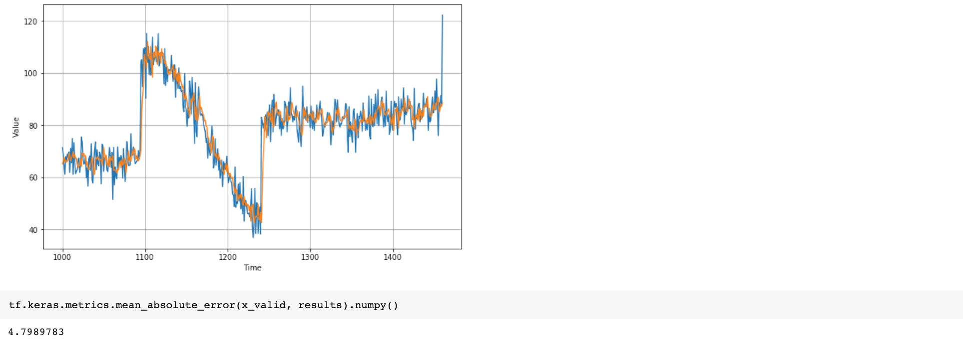

-w964

dataset = windowed_dataset(x_train, window_size, batch_size, shuffle_buffer_size)

model = tf.keras.models.Sequential([
    tf.keras.layers.Dense(10, input_shape=[window_size], activation="relu"), 
    tf.keras.layers.Dense(10, activation="relu"), 
    tf.keras.layers.Dense(1)
])

lr_schedule = tf.keras.callbacks.LearningRateScheduler(  # find the optimal learning rate | This will be called at the callback at the end of each epoch. It will change a learing rate to a value based on the epoch number
    lambda epoch: 1e-8 * 10**(epoch / 20))
optimizer = tf.keras.optimizers.SGD(lr=1e-8, momentum=0.9) #!!!!
model.compile(loss="mse", optimizer=optimizer)
history = model.fit(dataset, epochs=100, callbacks=[lr_schedule], verbose=0)

# -------------

lrs = 1e-8 * (10 ** (np.arange(100) / 20))
plt.semilogx(lrs, history.history["loss"])  # y-axis show the loss of that epoch, x-axis shows the learning rate
plt.axis([1e-8, 1e-3, 0, 300])   # stable right around 10^(-6)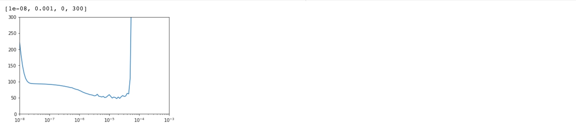

-w967 Use the best learning rate by observing the above plot

window_size = 30
dataset = windowed_dataset(x_train, window_size, batch_size, shuffle_buffer_size)

model = tf.keras.models.Sequential([
  tf.keras.layers.Dense(10, activation="relu", input_shape=[window_size]),
  tf.keras.layers.Dense(10, activation="relu"),
  tf.keras.layers.Dense(1)
])

optimizer = tf.keras.optimizers.SGD(lr=8e-6, momentum=0.9)
model.compile(loss="mse", optimizer=optimizer)
history = model.fit(dataset, epochs=500, verbose=0)

# ---------------

loss = history.history['loss']
epochs = range(len(loss))
plt.plot(epochs, loss, 'b', label='Training Loss')
plt.show()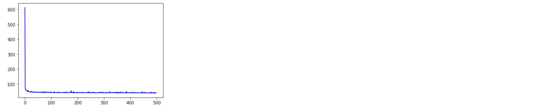

-w952

# Plot all but the first 10
loss = history.history['loss']
epochs = range(10, len(loss))
plot_loss = loss[10:]
print(plot_loss)
plt.plot(epochs, plot_loss, 'b', label='Training Loss')
plt.show()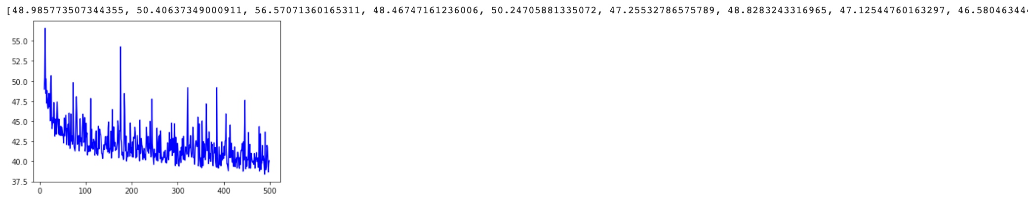

-w1041

forecast = []
for time in range(len(series) - window_size):
  forecast.append(model.predict(series[time:time + window_size][np.newaxis]))

forecast = forecast[split_time-window_size:]
results = np.array(forecast)[:, 0, 0]


plt.figure(figsize=(10, 6))

plot_series(time_valid, x_valid)
plot_series(time_valid, results)

print(tf.keras.metrics.mean_absolute_error(x_valid, results).numpy())
# 6.888425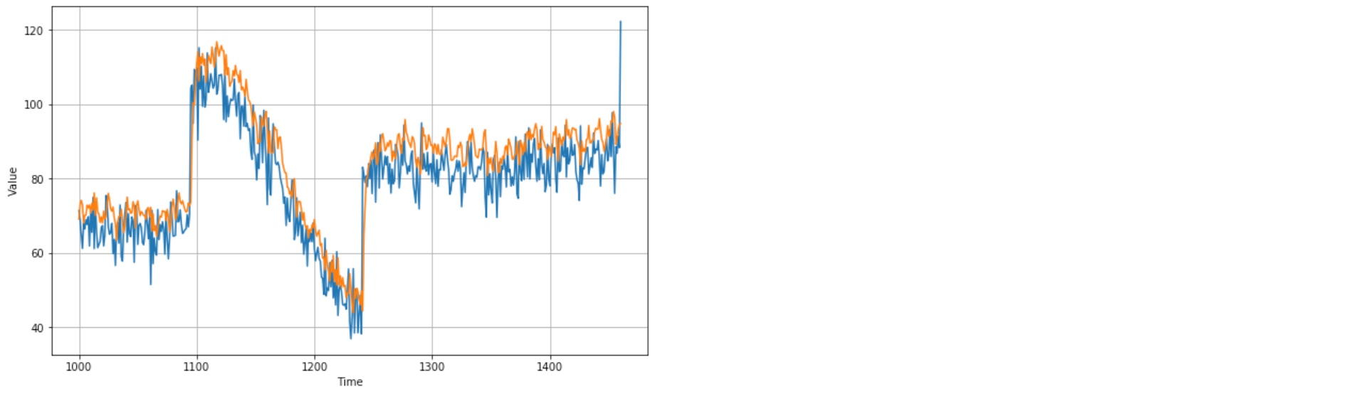

-w951

RNN for Time Series

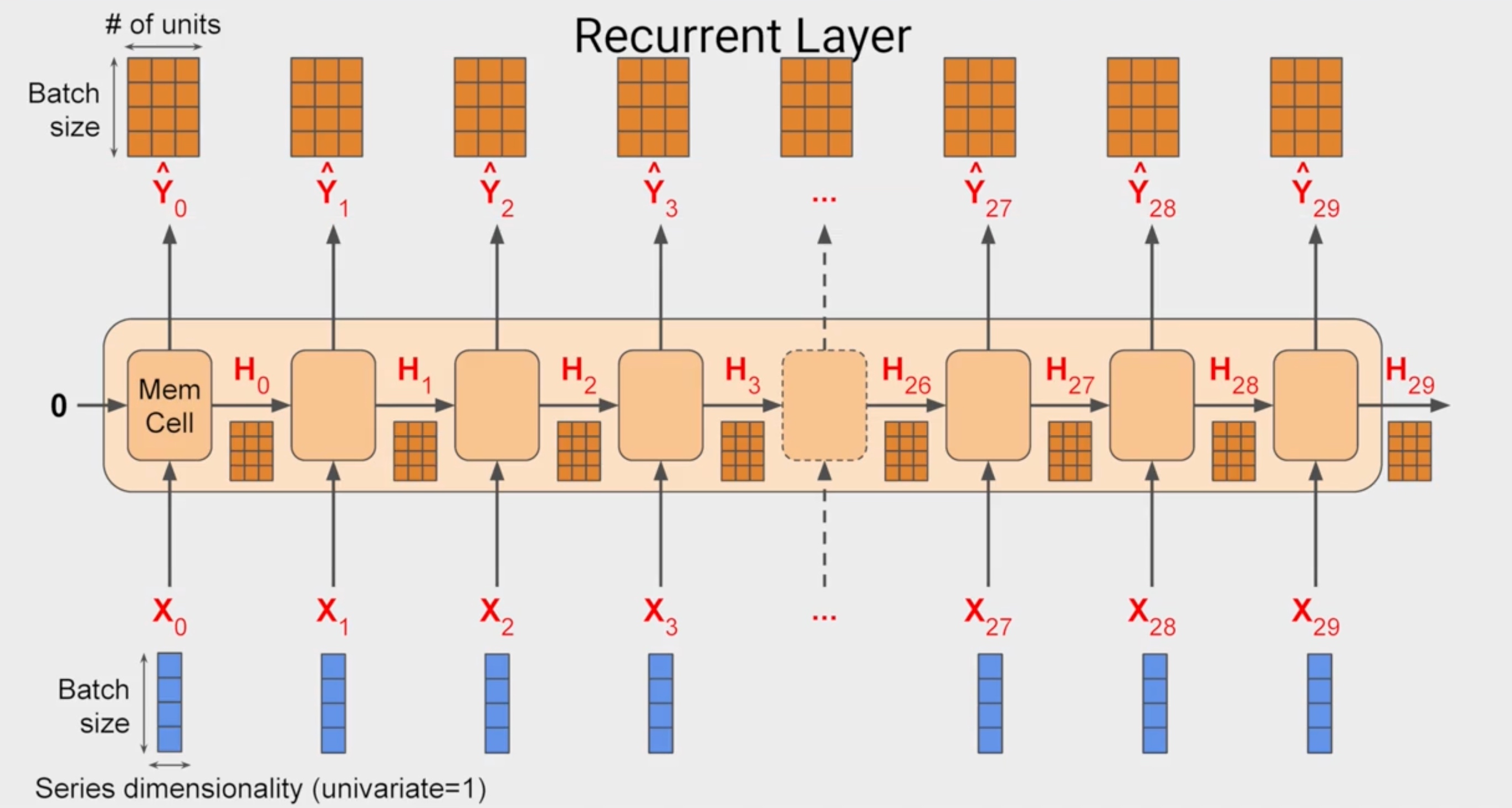
-w1368 -w1334 This is the default behaivour in keras. Can be changed by return_sequence=True

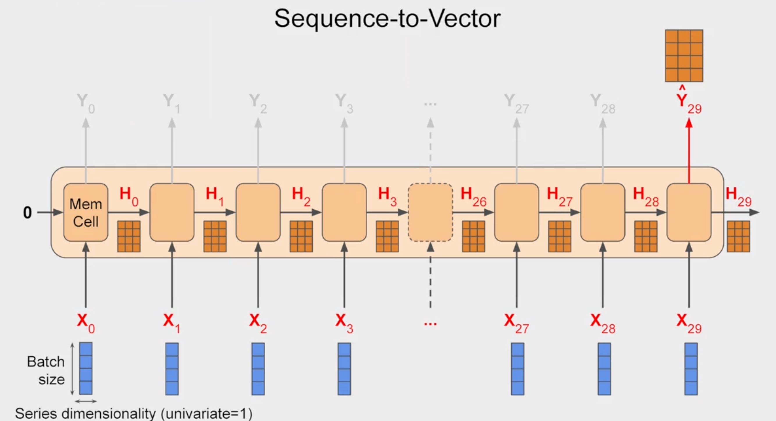
Sequence to Sequence RNN 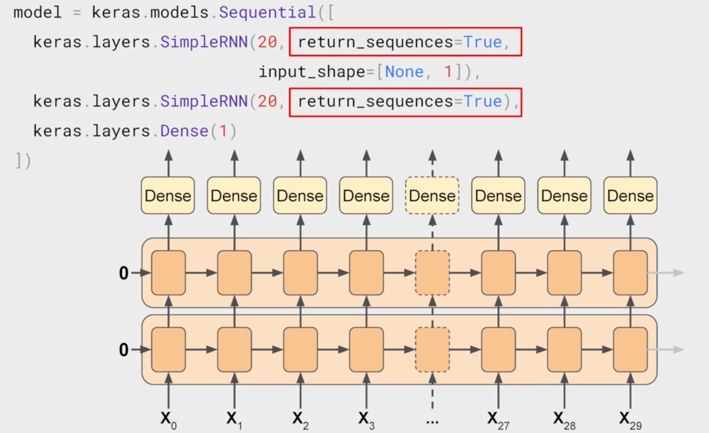-w1169 input shape can be [None,1]. It is None, since it is depended on batch size

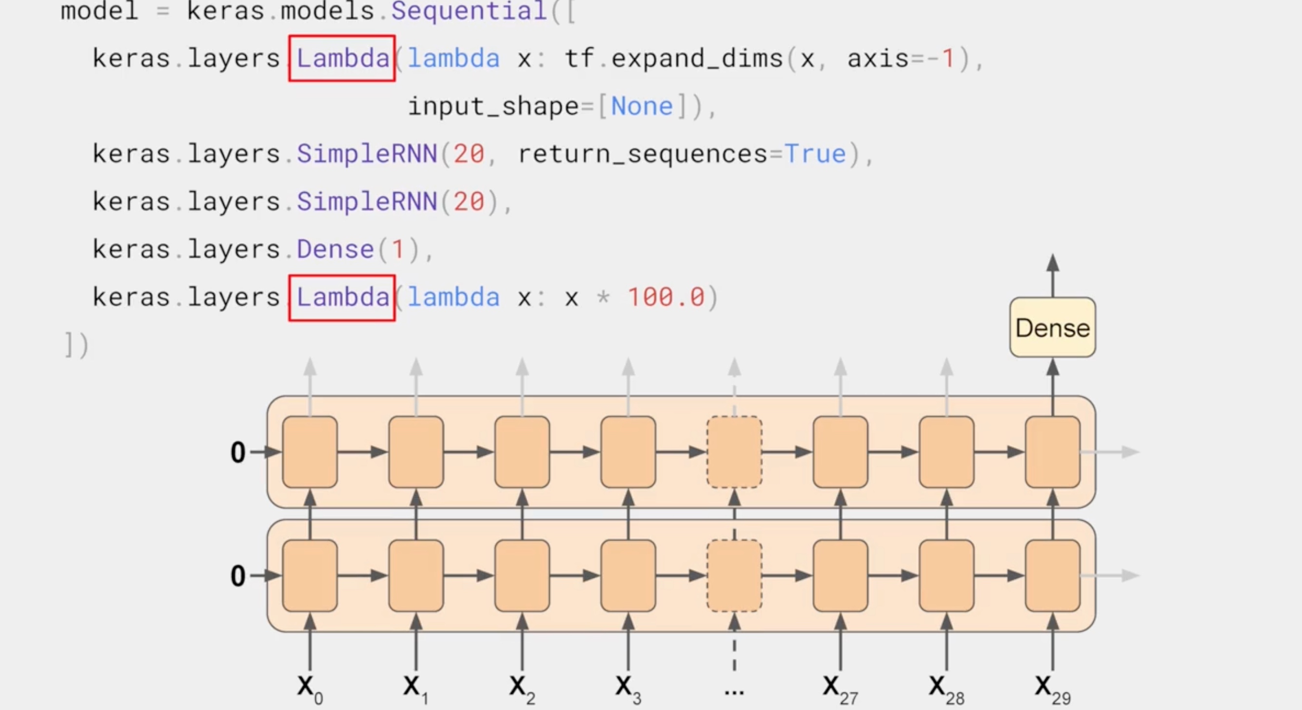
Lambda layer

This type of layer is one that allows to perform arbitrary operations to effectively expand functionality of Keras -w1335

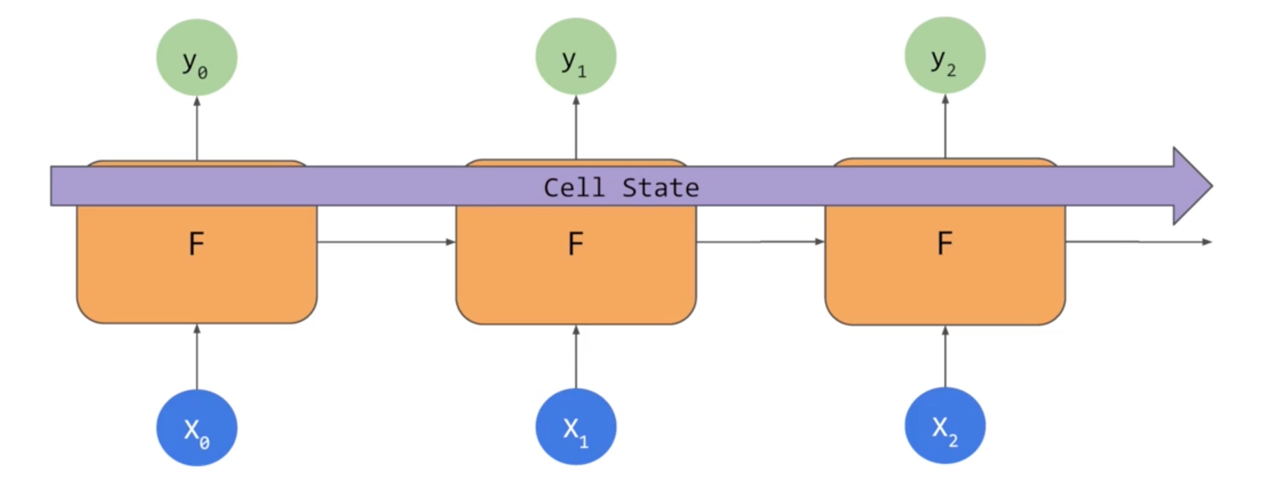
LSTM -w1244

SimpleRNN

%tensorflow_version 2.x
import tensorflow as tf
import numpy as np
import matplotlib.pyplot as plt
print(tf.__version__)

def plot_series(time, series, format="-", start=0, end=None):
    plt.plot(time[start:end], series[start:end], format)
    plt.xlabel("Time")
    plt.ylabel("Value")
    plt.grid(True)

def trend(time, slope=0):
    return slope * time

def seasonal_pattern(season_time):
    """Just an arbitrary pattern, you can change it if you wish"""
    return np.where(season_time < 0.4,
                    np.cos(season_time * 2 * np.pi),
                    1 / np.exp(3 * season_time))

def seasonality(time, period, amplitude=1, phase=0):
    """Repeats the same pattern at each period"""
    season_time = ((time + phase) % period) / period
    return amplitude * seasonal_pattern(season_time)

def noise(time, noise_level=1, seed=None):
    rnd = np.random.RandomState(seed)
    return rnd.randn(len(time)) * noise_level

time = np.arange(4 * 365 + 1, dtype="float32")
baseline = 10
series = trend(time, 0.1)  
baseline = 10
amplitude = 40
slope = 0.05
noise_level = 5

# Create the series
series = baseline + trend(time, slope) + seasonality(time, period=365, amplitude=amplitude)
# Update with noise
series += noise(time, noise_level, seed=42)

split_time = 1000
time_train = time[:split_time]
x_train = series[:split_time]
time_valid = time[split_time:]
x_valid = series[split_time:]

window_size = 20
batch_size = 32
shuffle_buffer_size = 1000

def windowed_dataset(series, window_size, batch_size, shuffle_buffer):
  dataset = tf.data.Dataset.from_tensor_slices(series)
  dataset = dataset.window(window_size + 1, shift=1, drop_remainder=True)
  dataset = dataset.flat_map(lambda window: window.batch(window_size + 1))
  dataset = dataset.shuffle(shuffle_buffer).map(lambda window: (window[:-1], window[-1]))
  dataset = dataset.batch(batch_size).prefetch(1)
  return dataset

Find the optimal learning rate

tf.keras.backend.clear_session()
tf.random.set_seed(51)
np.random.seed(51)

train_set = windowed_dataset(x_train, window_size, batch_size=128, shuffle_buffer=shuffle_buffer_size)

model = tf.keras.models.Sequential([
  tf.keras.layers.Lambda(lambda x: tf.expand_dims(x, axis=-1), # tf.expand_dims changes the shape by adding 1 to dimensions. For example, a vector with 10 elements could be treated as a 10x1 matrix.
                      input_shape=[None]),
  tf.keras.layers.SimpleRNN(40, return_sequences=True), 
  tf.keras.layers.SimpleRNN(40),
  tf.keras.layers.Dense(1),
  tf.keras.layers.Lambda(lambda x: x * 100.0)
])

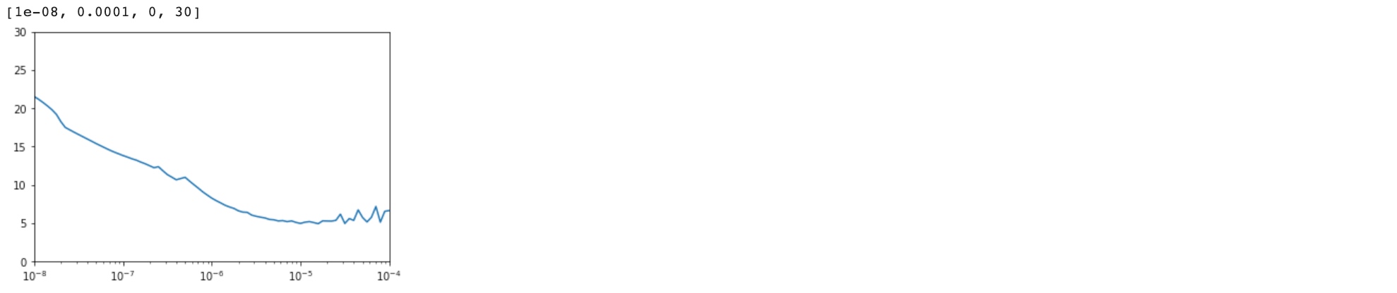
lr_schedule = tf.keras.callbacks.LearningRateScheduler(
    lambda epoch: 1e-8 * 10**(epoch / 20))
optimizer = tf.keras.optimizers.SGD(lr=1e-8, momentum=0.9)
model.compile(loss=tf.keras.losses.Huber(),
              optimizer=optimizer,
              metrics=["mae"])
history = model.fit(train_set, epochs=100, callbacks=[lr_schedule])


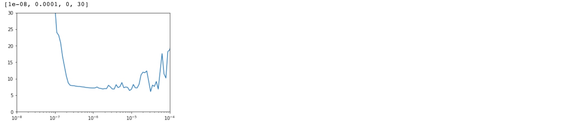
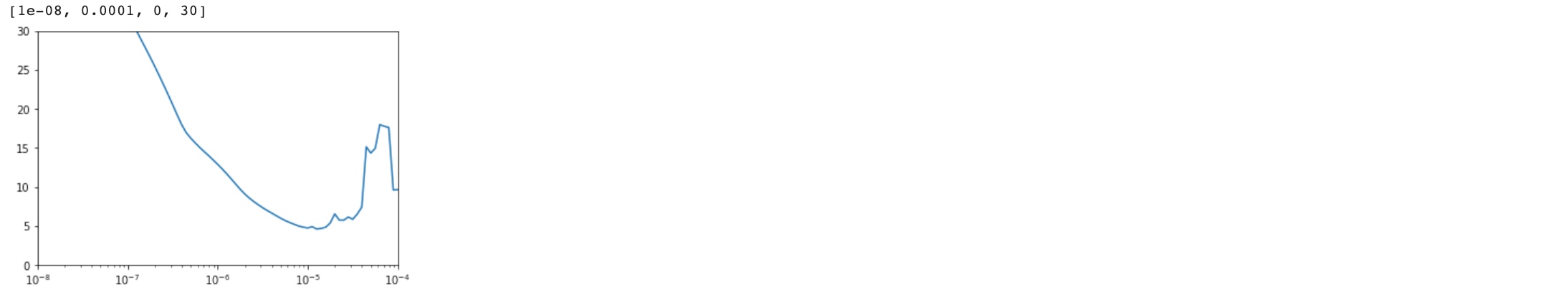
plt.semilogx(history.history["lr"], history.history["loss"])
plt.axis([1e-8, 1e-4, 0, 30])

-w1151 -w965

Use the optimal learning rate

tf.keras.backend.clear_session()
tf.random.set_seed(51)
np.random.seed(51)

dataset = windowed_dataset(x_train, window_size, batch_size=128, shuffle_buffer=shuffle_buffer_size)

model = tf.keras.models.Sequential([
  tf.keras.layers.Lambda(lambda x: tf.expand_dims(x, axis=-1),
                      input_shape=[None]),
  tf.keras.layers.SimpleRNN(40, return_sequences=True),
  tf.keras.layers.SimpleRNN(40),
  tf.keras.layers.Dense(1),
  tf.keras.layers.Lambda(lambda x: x * 100.0)
])

optimizer = tf.keras.optimizers.SGD(lr=5e-5, momentum=0.9)
model.compile(loss=tf.keras.losses.Huber(),   # huber loss function which less sensitive to outliers 
              optimizer=optimizer,
              metrics=["mae"])
history = model.fit(dataset,epochs=400)

-w1110

forecast=[]
for time in range(len(series) - window_size):
  forecast.append(model.predict(series[time:time + window_size][np.newaxis]))

forecast = forecast[split_time-window_size:]
results = np.array(forecast)[:, 0, 0]


plt.figure(figsize=(10, 6))

plot_series(time_valid, x_valid)
plot_series(time_valid, results)

print(tf.keras.metrics.mean_absolute_error(x_valid, results).numpy())
# 6.129704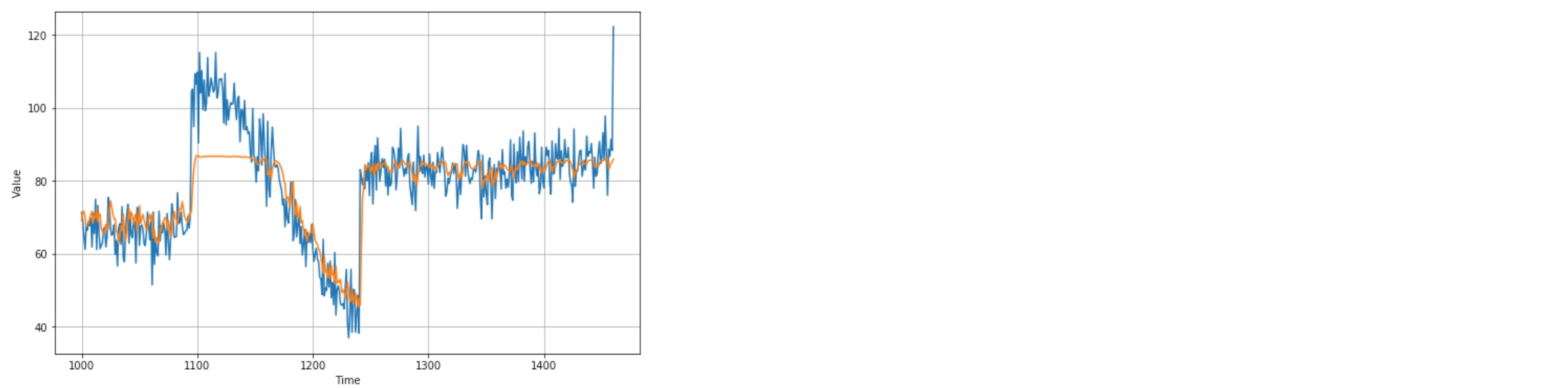

-w1122

import matplotlib.image  as mpimg
import matplotlib.pyplot as plt

#-----------------------------------------------------------
# Retrieve a list of list results on training and test data
# sets for each training epoch
#-----------------------------------------------------------
mae=history.history['mae']
loss=history.history['loss']

epochs=range(len(loss)) # Get number of epochs

#------------------------------------------------
# Plot MAE and Loss
#------------------------------------------------
plt.plot(epochs, mae, 'r')
plt.plot(epochs, loss, 'b')
plt.title('MAE and Loss')
plt.xlabel("Epochs")
plt.ylabel("Accuracy")
plt.legend(["MAE", "Loss"])

plt.figure()

epochs_zoom = epochs[200:]
mae_zoom = mae[200:]
loss_zoom = loss[200:]

#------------------------------------------------
# Plot Zoomed MAE and Loss
#------------------------------------------------
plt.plot(epochs_zoom, mae_zoom, 'r')
plt.plot(epochs_zoom, loss_zoom, 'b')
plt.title('MAE and Loss')
plt.xlabel("Epochs")
plt.ylabel("Accuracy")
plt.legend(["MAE", "Loss"])

plt.figure()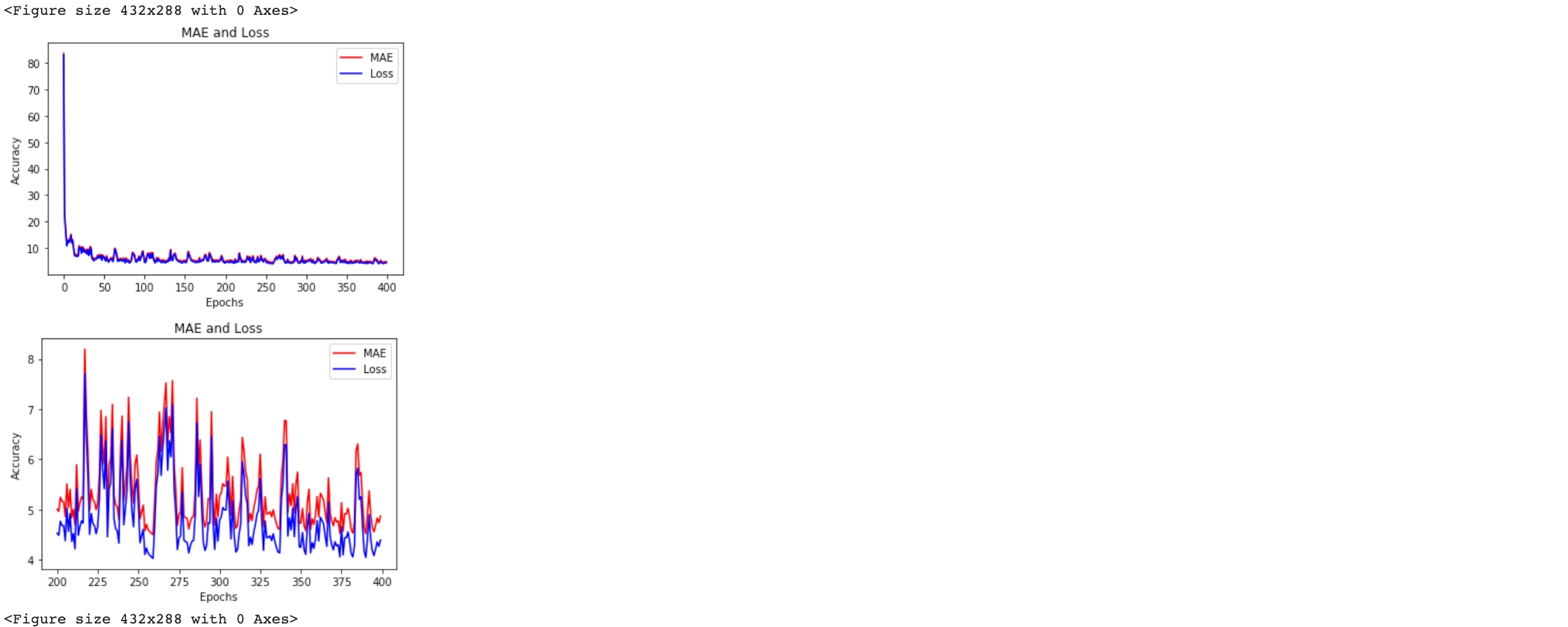

-w1107

Multi layer LSTM

find optimal learning rate

tf.keras.backend.clear_session()  # clear any internal variable
tf.random.set_seed(51)
np.random.seed(51)

tf.keras.backend.clear_session()
dataset = windowed_dataset(x_train, window_size, batch_size, shuffle_buffer_size)

model = tf.keras.models.Sequential([
  tf.keras.layers.Lambda(lambda x: tf.expand_dims(x, axis=-1),
                      input_shape=[None]),
    tf.keras.layers.Bidirectional(tf.keras.layers.LSTM(32, return_sequences=True)),
  tf.keras.layers.Bidirectional(tf.keras.layers.LSTM(32)),
  tf.keras.layers.Dense(1),
  tf.keras.layers.Lambda(lambda x: x * 100.0)
])

lr_schedule = tf.keras.callbacks.LearningRateScheduler(
    lambda epoch: 1e-8 * 10**(epoch / 20))
optimizer = tf.keras.optimizers.SGD(lr=1e-8, momentum=0.9)
model.compile(loss=tf.keras.losses.Huber(),
              optimizer=optimizer,
              metrics=["mae"])
history = model.fit(dataset, epochs=100, callbacks=[lr_schedule])

plt.semilogx(history.history["lr"], history.history["loss"])
plt.axis([1e-8, 1e-4, 0, 30])

-w1028 -w989

Use optimal learning rate

tf.keras.backend.clear_session()
tf.random.set_seed(51)
np.random.seed(51)

tf.keras.backend.clear_session()
dataset = windowed_dataset(x_train, window_size, batch_size, shuffle_buffer_size)

model = tf.keras.models.Sequential([
  tf.keras.layers.Lambda(lambda x: tf.expand_dims(x, axis=-1),
                      input_shape=[None]),
   tf.keras.layers.Bidirectional(tf.keras.layers.LSTM(32, return_sequences=True)),
  tf.keras.layers.Bidirectional(tf.keras.layers.LSTM(32)),
  tf.keras.layers.Dense(1),
  tf.keras.layers.Lambda(lambda x: x * 100.0)
])


model.compile(loss="mse", optimizer=tf.keras.optimizers.SGD(lr=1e-5, momentum=0.9),metrics=["mae"])
history = model.fit(dataset,epochs=500,verbose=0)

forecast = []
results = []
for time in range(len(series) - window_size):
  forecast.append(model.predict(series[time:time + window_size][np.newaxis]))

forecast = forecast[split_time-window_size:]
results = np.array(forecast)[:, 0, 0]


plt.figure(figsize=(10, 6))

plot_series(time_valid, x_valid)
plot_series(time_valid, results)

print(tf.keras.metrics.mean_absolute_error(x_valid, results).numpy())
# 6.6017175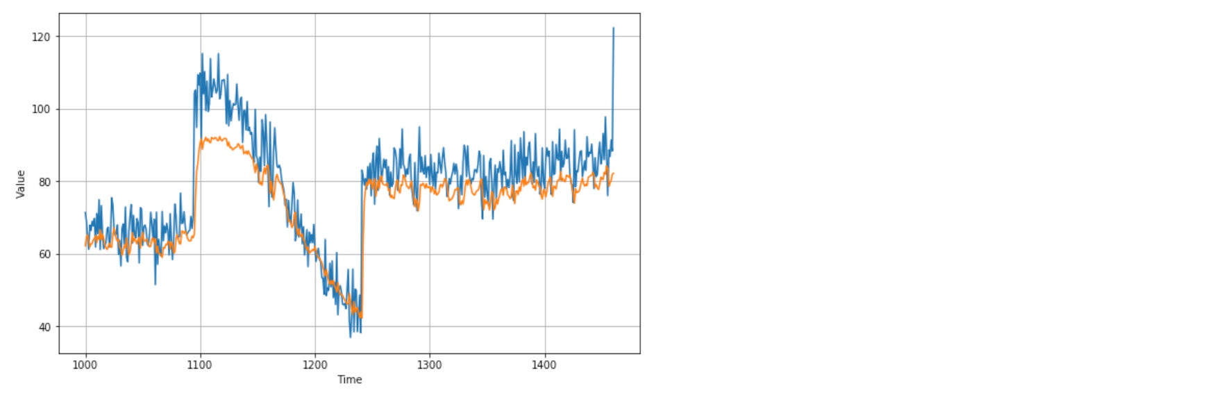

-w878

import matplotlib.image  as mpimg
import matplotlib.pyplot as plt

#-----------------------------------------------------------
# Retrieve a list of list results on training and test data
# sets for each training epoch
#-----------------------------------------------------------
mae=history.history['mae']
loss=history.history['loss']

epochs=range(len(loss)) # Get number of epochs

#------------------------------------------------
# Plot MAE and Loss
#------------------------------------------------
plt.plot(epochs, mae, 'r')
plt.plot(epochs, loss, 'b')
plt.title('MAE and Loss')
plt.xlabel("Epochs")
plt.ylabel("Accuracy")
plt.legend(["MAE", "Loss"])

plt.figure()

epochs_zoom = epochs[200:]
mae_zoom = mae[200:]
loss_zoom = loss[200:]

#------------------------------------------------
# Plot Zoomed MAE and Loss
#------------------------------------------------
plt.plot(epochs_zoom, mae_zoom, 'r')
plt.plot(epochs_zoom, loss_zoom, 'b')
plt.title('MAE and Loss')
plt.xlabel("Epochs")
plt.ylabel("Accuracy")
plt.legend(["MAE", "Loss"])

plt.figure()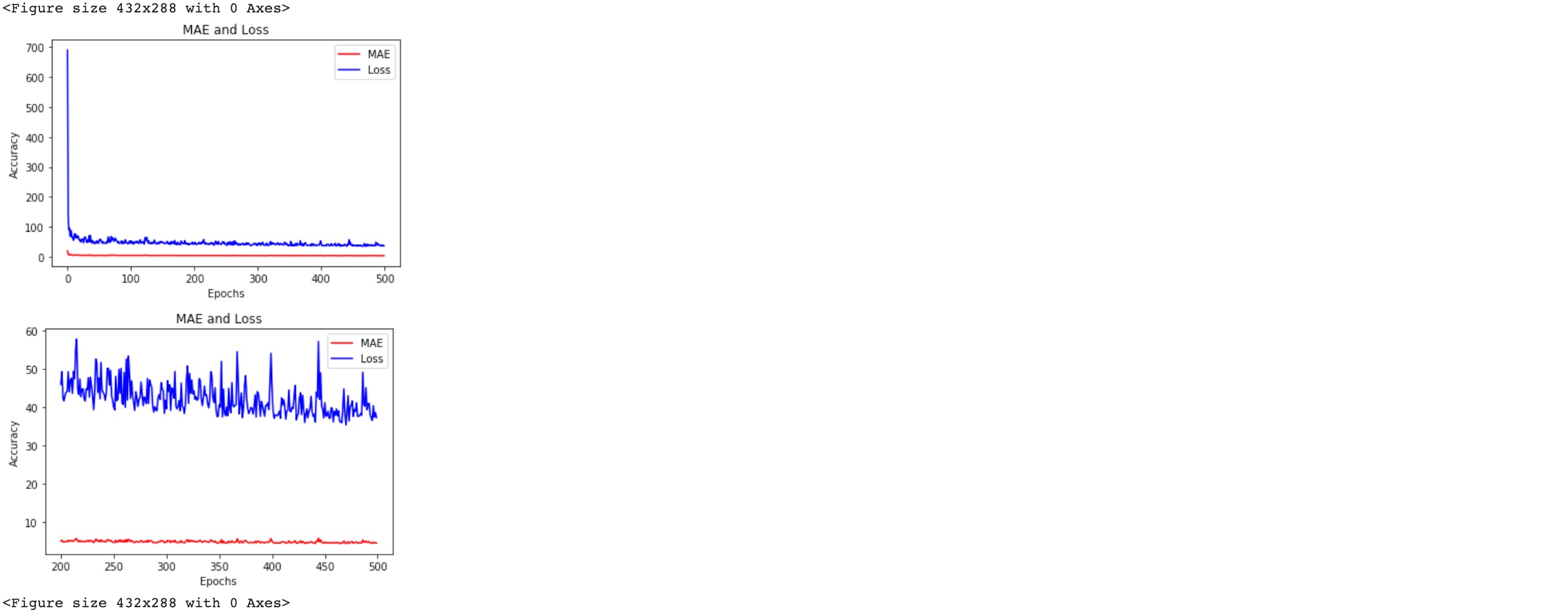

-w1132

Triple LSTM layer

tf.keras.backend.clear_session()
dataset = windowed_dataset(x_train, window_size, batch_size, shuffle_buffer_size)

model = tf.keras.models.Sequential([
  tf.keras.layers.Lambda(lambda x: tf.expand_dims(x, axis=-1),
                      input_shape=[None]),
  tf.keras.layers.Bidirectional(tf.keras.layers.LSTM(32, return_sequences=True)),
  tf.keras.layers.Bidirectional(tf.keras.layers.LSTM(32, return_sequences=True)),
  tf.keras.layers.Bidirectional(tf.keras.layers.LSTM(32)),
  tf.keras.layers.Dense(1),
  tf.keras.layers.Lambda(lambda x: x * 100.0)
])


model.compile(loss="mse", optimizer=tf.keras.optimizers.SGD(lr=1e-6, momentum=0.9))
model.fit(dataset,epochs=100)

-w913

forecast = []
results = []
for time in range(len(series) - window_size):
  forecast.append(model.predict(series[time:time + window_size][np.newaxis]))

forecast = forecast[split_time-window_size:]
results = np.array(forecast)[:, 0, 0]


plt.figure(figsize=(10, 6))

plot_series(time_valid, x_valid)
plot_series(time_valid, results)

tf.keras.metrics.mean_absolute_error(x_valid, results).numpy()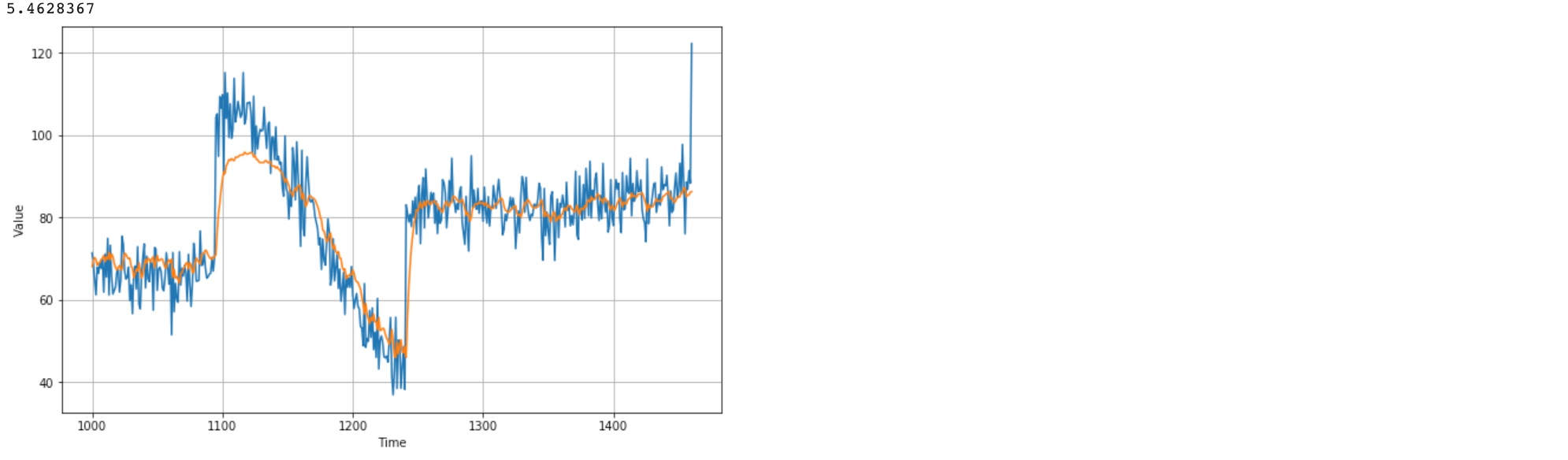

-w995

Real World Time Series

%tensorflow_version 2.x

import tensorflow as tf
import numpy as np
import matplotlib.pyplot as plt
print(tf.__version__)

def plot_series(time, series, format="-", start=0, end=None):
    plt.plot(time[start:end], series[start:end], format)
    plt.xlabel("Time")
    plt.ylabel("Value")
    plt.grid(True)

def trend(time, slope=0):
    return slope * time

def seasonal_pattern(season_time):
    """Just an arbitrary pattern, you can change it if you wish"""
    return np.where(season_time < 0.4,
                    np.cos(season_time * 2 * np.pi),
                    1 / np.exp(3 * season_time))

def seasonality(time, period, amplitude=1, phase=0):
    """Repeats the same pattern at each period"""
    season_time = ((time + phase) % period) / period
    return amplitude * seasonal_pattern(season_time)

def noise(time, noise_level=1, seed=None):
    rnd = np.random.RandomState(seed)
    return rnd.randn(len(time)) * noise_level

time = np.arange(4 * 365 + 1, dtype="float32")
baseline = 10
series = trend(time, 0.1)  
baseline = 10
amplitude = 40
slope = 0.05
noise_level = 5

# Create the series
series = baseline + trend(time, slope) + seasonality(time, period=365, amplitude=amplitude)
# Update with noise
series += noise(time, noise_level, seed=42)

split_time = 1000
time_train = time[:split_time]
x_train = series[:split_time]
time_valid = time[split_time:]
x_valid = series[split_time:]

window_size = 20
batch_size = 32
shuffle_buffer_size = 1000

def windowed_dataset(series, window_size, batch_size, shuffle_buffer):
    series = tf.expand_dims(series, axis=-1)  # !!!!!!!!
    ds = tf.data.Dataset.from_tensor_slices(series)
    ds = ds.window(window_size + 1, shift=1, drop_remainder=True)
    ds = ds.flat_map(lambda w: w.batch(window_size + 1))
    ds = ds.shuffle(shuffle_buffer)
    ds = ds.map(lambda w: (w[:-1], w[1:]))
    return ds.batch(batch_size).prefetch(1)

# -----------------

def model_forecast(model, series, window_size):
    ds = tf.data.Dataset.from_tensor_slices(series)
    ds = ds.window(window_size, shift=1, drop_remainder=True)
    ds = ds.flat_map(lambda w: w.batch(window_size))
    ds = ds.batch(32).prefetch(1)
    forecast = model.predict(ds)
    return forecast

tf.keras.backend.clear_session()
tf.random.set_seed(51)
np.random.seed(51)

window_size = 30
train_set = windowed_dataset(x_train, window_size, batch_size=128, shuffle_buffer=shuffle_buffer_size)

model = tf.keras.models.Sequential([
  tf.keras.layers.Conv1D(filters=32, kernel_size=5,
                      strides=1, padding="causal",
                      activation="relu",
                      input_shape=[None, 1]),
  tf.keras.layers.Bidirectional(tf.keras.layers.LSTM(32, return_sequences=True)),
  tf.keras.layers.Bidirectional(tf.keras.layers.LSTM(32, return_sequences=True)),
  tf.keras.layers.Dense(1),
  tf.keras.layers.Lambda(lambda x: x * 200)
])
lr_schedule = tf.keras.callbacks.LearningRateScheduler(
    lambda epoch: 1e-8 * 10**(epoch / 20))
optimizer = tf.keras.optimizers.SGD(lr=1e-8, momentum=0.9)
model.compile(loss=tf.keras.losses.Huber(),
              optimizer=optimizer,
              metrics=["mae"])
history = model.fit(train_set, epochs=100, callbacks=[lr_schedule])


plt.semilogx(history.history["lr"], history.history["loss"])
plt.axis([1e-8, 1e-4, 0, 30])

-w1034 -w1094

tf.keras.backend.clear_session()
tf.random.set_seed(51)
np.random.seed(51)
#batch_size = 16
dataset = windowed_dataset(x_train, window_size, batch_size, shuffle_buffer_size)

model = tf.keras.models.Sequential([
  tf.keras.layers.Conv1D(filters=32, kernel_size=3,
                      strides=1, padding="causal",
                      activation="relu",
                      input_shape=[None, 1]),
  tf.keras.layers.LSTM(32, return_sequences=True),
  tf.keras.layers.LSTM(32, return_sequences=True),
  tf.keras.layers.Dense(1),
  tf.keras.layers.Lambda(lambda x: x * 200)
])

optimizer = tf.keras.optimizers.SGD(lr=1e-5, momentum=0.9)
model.compile(loss=tf.keras.losses.Huber(),
              optimizer=optimizer,
              metrics=["mae"])
history = model.fit(dataset,epochs=500)

-w1013

rnn_forecast = model_forecast(model, series[..., np.newaxis], window_size)
rnn_forecast = rnn_forecast[split_time - window_size:-1, -1, 0]


plt.figure(figsize=(10, 6))
plot_series(time_valid, x_valid)
plot_series(time_valid, rnn_forecast)


print(tf.keras.metrics.mean_absolute_error(x_valid, rnn_forecast).numpy())
# 5.0638213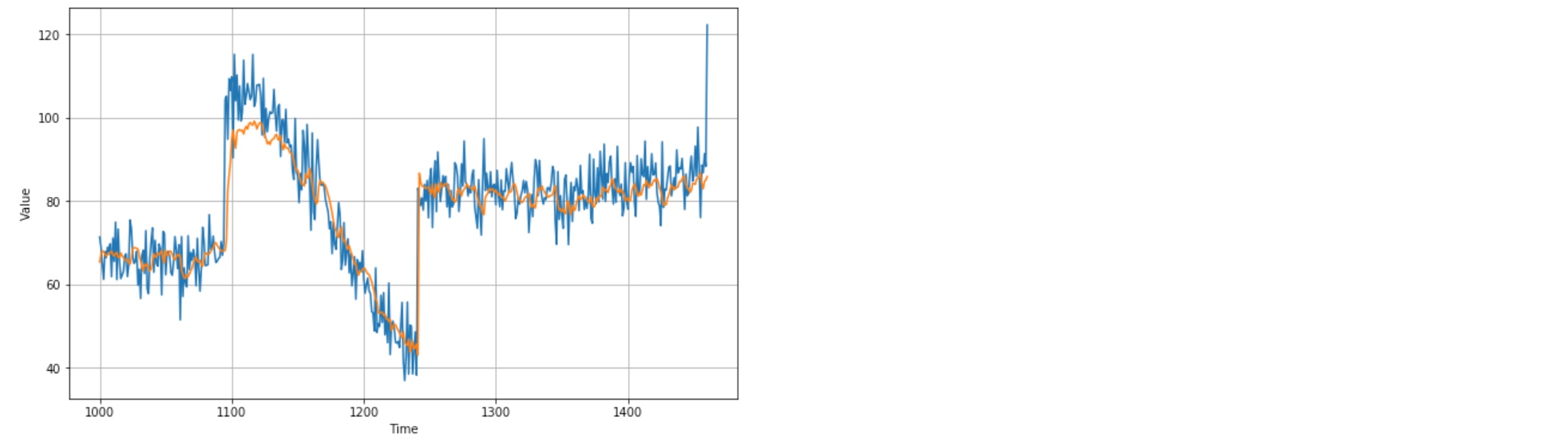

-w982

import matplotlib.image  as mpimg
import matplotlib.pyplot as plt

#-----------------------------------------------------------
# Retrieve a list of list results on training and test data
# sets for each training epoch
#-----------------------------------------------------------
mae=history.history['mae']
loss=history.history['loss']

epochs=range(len(loss)) # Get number of epochs

#------------------------------------------------
# Plot MAE and Loss
#------------------------------------------------
plt.plot(epochs, mae, 'r')
plt.plot(epochs, loss, 'b')
plt.title('MAE and Loss')
plt.xlabel("Epochs")
plt.ylabel("Accuracy")
plt.legend(["MAE", "Loss"])

plt.figure()

epochs_zoom = epochs[200:]
mae_zoom = mae[200:]
loss_zoom = loss[200:]

#------------------------------------------------
# Plot Zoomed MAE and Loss
#------------------------------------------------
plt.plot(epochs_zoom, mae_zoom, 'r')
plt.plot(epochs_zoom, loss_zoom, 'b')
plt.title('MAE and Loss')
plt.xlabel("Epochs")
plt.ylabel("Accuracy")
plt.legend(["MAE", "Loss"])

plt.figure()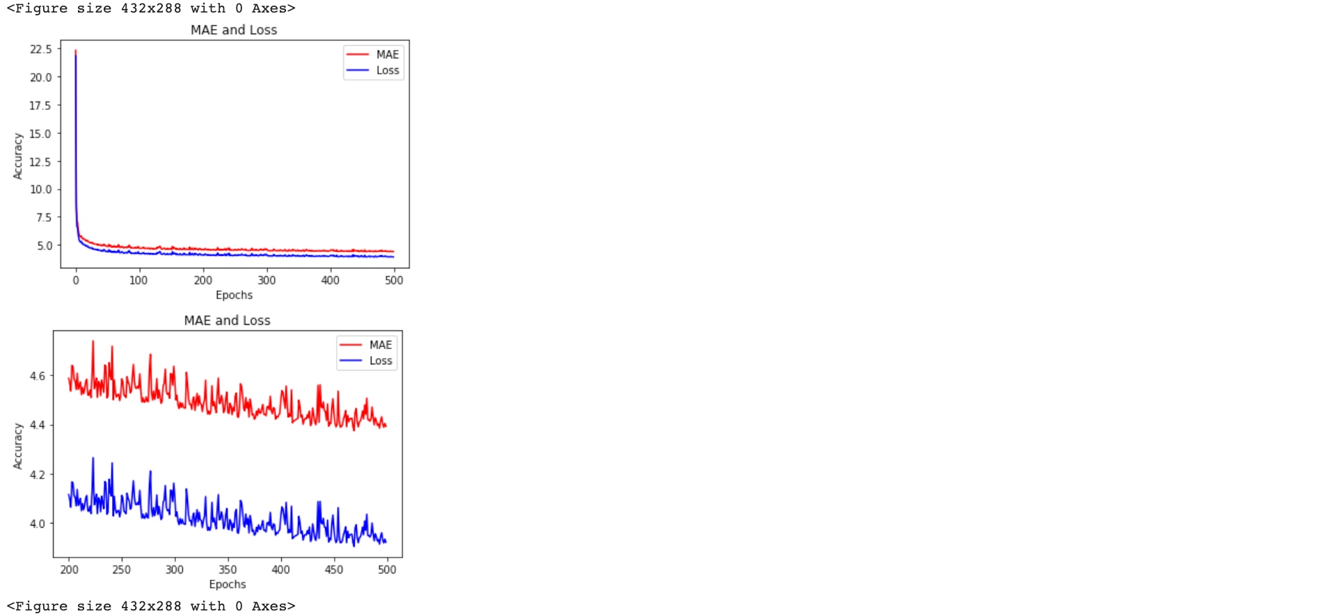

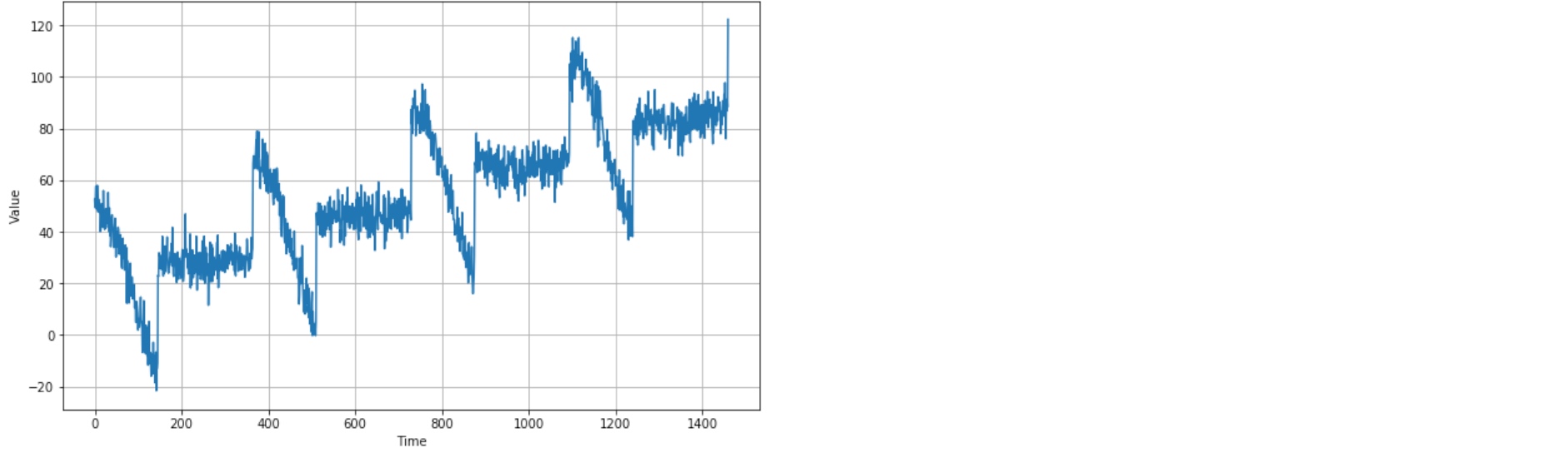
-w947

Sunspot Dataset

Monthly Mean Total Sunspot Number - form 1749 to july 2018 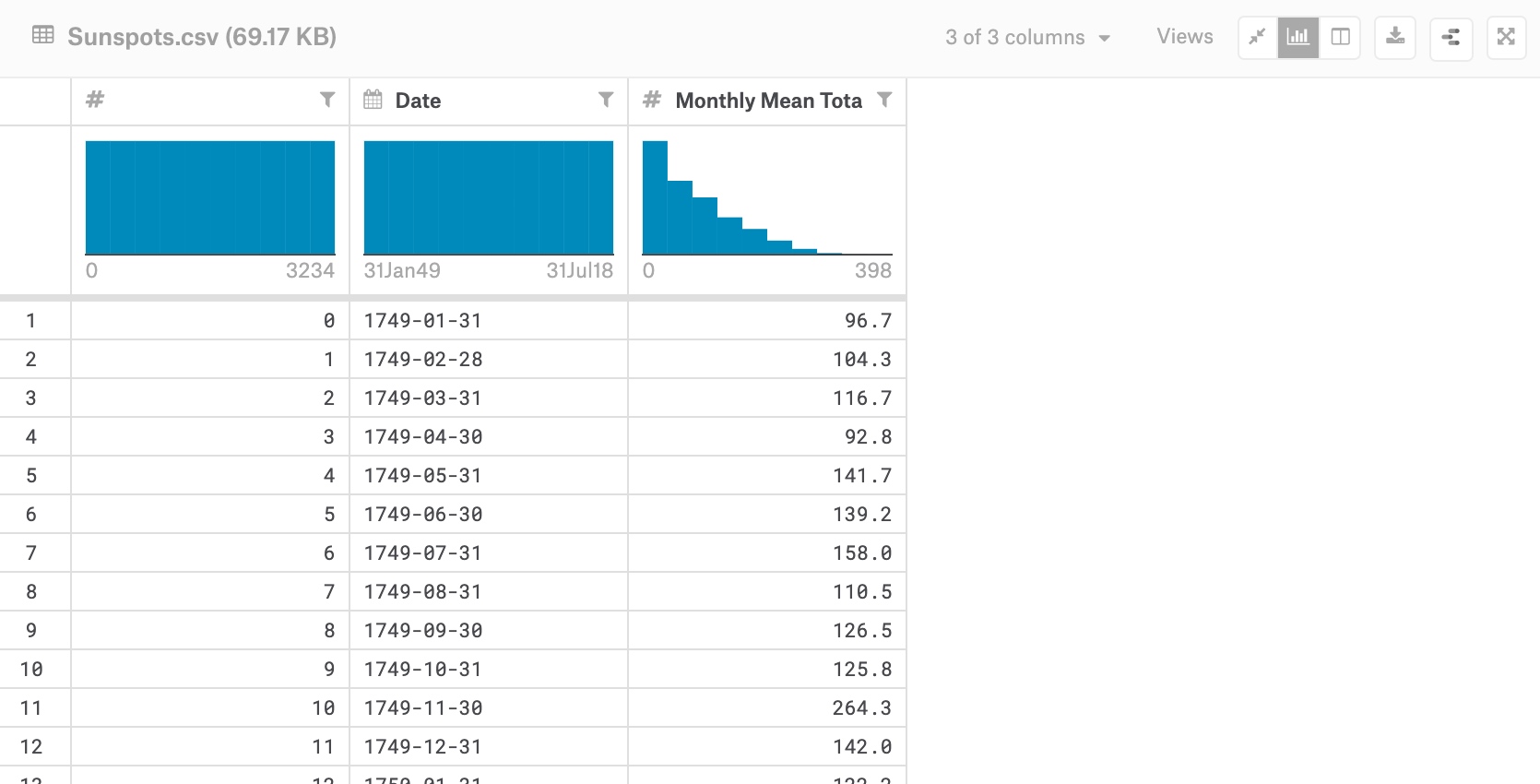-w835 Sunspots usually appear in pairs of opposite magnetic polarity. Their number varies according to the approximately 11-year solar cycle.

%tensorflow_version 2.x

import tensorflow as tf
print(tf.__version__)

import numpy as np
import matplotlib.pyplot as plt
def plot_series(time, series, format="-", start=0, end=None):
    plt.plot(time[start:end], series[start:end], format)
    plt.xlabel("Time")
    plt.ylabel("Value")
    plt.grid(True)


!wget --no-check-certificate \
    https://storage.googleapis.com/laurencemoroney-blog.appspot.com/Sunspots.csv \
    -O /tmp/sunspots.csv

import csv
time_step = []
sunspots = []

with open('/tmp/sunspots.csv') as csvfile:
  reader = csv.reader(csvfile, delimiter=',')
  next(reader)  # skip col titile
  for row in reader:
    sunspots.append(float(row[2])) # value (series)
    time_step.append(int(row[0])) # time step

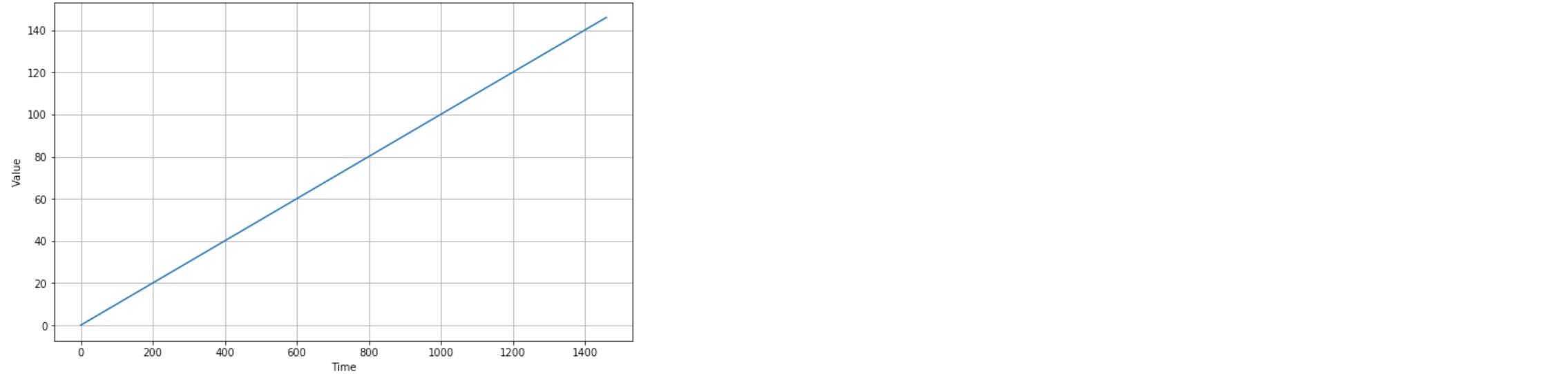
series = np.array(sunspots)
time = np.array(time_step)
plt.figure(figsize=(10, 6))
plot_series(time, series)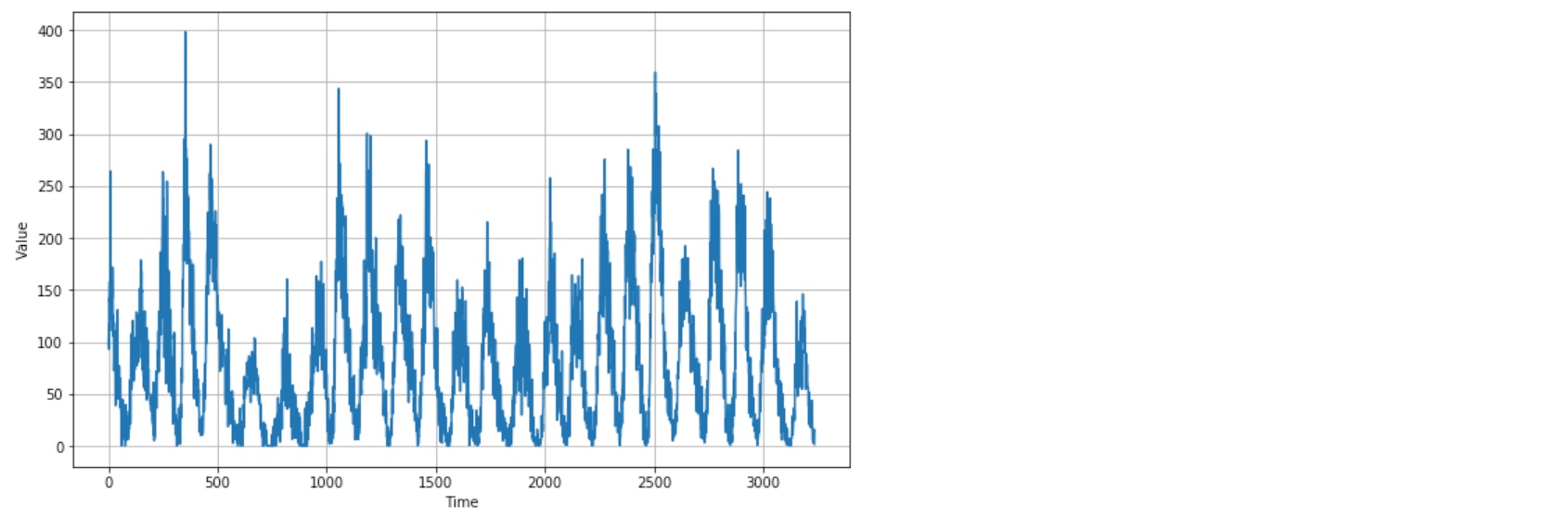

-w845

split_time = 3000
time_train = time[:split_time]
x_train = series[:split_time]
time_valid = time[split_time:]
x_valid = series[split_time:]

window_size = 30  # !!!!!!!
batch_size = 32
shuffle_buffer_size = 1000

change the data into windows dataset

def windowed_dataset(series, window_size, batch_size, shuffle_buffer):
    series = tf.expand_dims(series, axis=-1)
    ds = tf.data.Dataset.from_tensor_slices(series)
    ds = ds.window(window_size + 1, shift=1, drop_remainder=True)
    ds = ds.flat_map(lambda w: w.batch(window_size + 1))
    ds = ds.shuffle(shuffle_buffer)
    ds = ds.map(lambda w: (w[:-1], w[1:]))
    return ds.batch(batch_size).prefetch(1)

def model_forecast(model, series, window_size):
    ds = tf.data.Dataset.from_tensor_slices(series)
    ds = ds.window(window_size, shift=1, drop_remainder=True)
    ds = ds.flat_map(lambda w: w.batch(window_size))
    ds = ds.batch(32).prefetch(1)
    forecast = model.predict(ds)
    return forecast

tf.keras.backend.clear_session()
tf.random.set_seed(51)
np.random.seed(51)
window_size = 64
batch_size = 256
train_set = windowed_dataset(x_train, window_size, batch_size, shuffle_buffer_size)
print(train_set)
print(x_train.shape)

model = tf.keras.models.Sequential([
  tf.keras.layers.Conv1D(filters=32, kernel_size=5,
                      strides=1, padding="causal",
                      activation="relu",
                      input_shape=[None, 1]),
  tf.keras.layers.LSTM(64, return_sequences=True),
  tf.keras.layers.LSTM(64, return_sequences=True),
  tf.keras.layers.Dense(30, activation="relu"),
  tf.keras.layers.Dense(10, activation="relu"),
  tf.keras.layers.Dense(1),
  tf.keras.layers.Lambda(lambda x: x * 400)  # the value range is b/w 1 and 318.56
])

lr_schedule = tf.keras.callbacks.LearningRateScheduler(
    lambda epoch: 1e-8 * 10**(epoch / 20))
optimizer = tf.keras.optimizers.SGD(lr=1e-8, momentum=0.9)
model.compile(loss=tf.keras.losses.Huber(),
              optimizer=optimizer,
              metrics=["mae"])
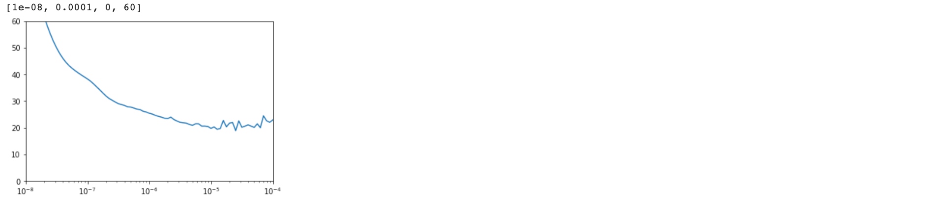
history = model.fit(train_set, epochs=100, callbacks=[lr_schedule])


plt.semilogx(history.history["lr"], history.history["loss"])
plt.axis([1e-8, 1e-4, 0, 60])

-w1095 -w943

LSTM:

tf.keras.backend.clear_session()
tf.random.set_seed(51)
np.random.seed(51)
train_set = windowed_dataset(x_train, window_size=60, batch_size=100, shuffle_buffer=shuffle_buffer_size)
model = tf.keras.models.Sequential([
  tf.keras.layers.Conv1D(filters=60, kernel_size=5,
                      strides=1, padding="causal",
                      activation="relu",
                      input_shape=[None, 1]),
  tf.keras.layers.LSTM(60, return_sequences=True),
  tf.keras.layers.LSTM(60, return_sequences=True),
  tf.keras.layers.Dense(30, activation="relu"),
  tf.keras.layers.Dense(10, activation="relu"),
  tf.keras.layers.Dense(1),
  tf.keras.layers.Lambda(lambda x: x * 400)
])


optimizer = tf.keras.optimizers.SGD(lr=1e-5, momentum=0.9)
model.compile(loss=tf.keras.losses.Huber(),
              optimizer=optimizer,
              metrics=["mae"])
history = model.fit(train_set,epochs=500)

-w1044

rnn_forecast = model_forecast(model, series[..., np.newaxis], window_size)
rnn_forecast = rnn_forecast[split_time - window_size:-1, -1, 0]



plt.figure(figsize=(10, 6))
plot_series(time_valid, x_valid)
plot_series(time_valid, rnn_forecast)


print(tf.keras.metrics.mean_absolute_error(x_valid, rnn_forecast).numpy())
# 16.465754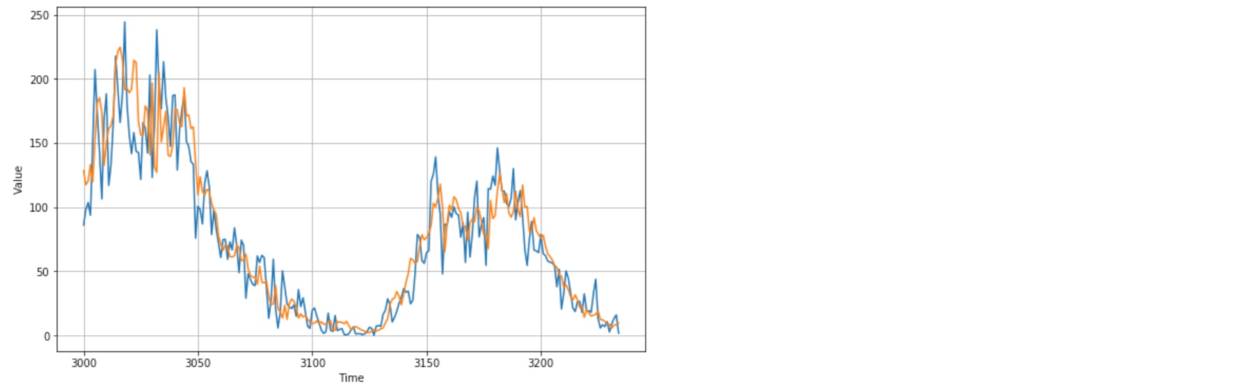

-w886

import matplotlib.image  as mpimg
import matplotlib.pyplot as plt

#-----------------------------------------------------------
# Retrieve a list of list results on training and test data
# sets for each training epoch
#-----------------------------------------------------------
loss=history.history['loss']

epochs=range(len(loss)) # Get number of epochs


#------------------------------------------------
# Plot training and validation loss per epoch
#------------------------------------------------
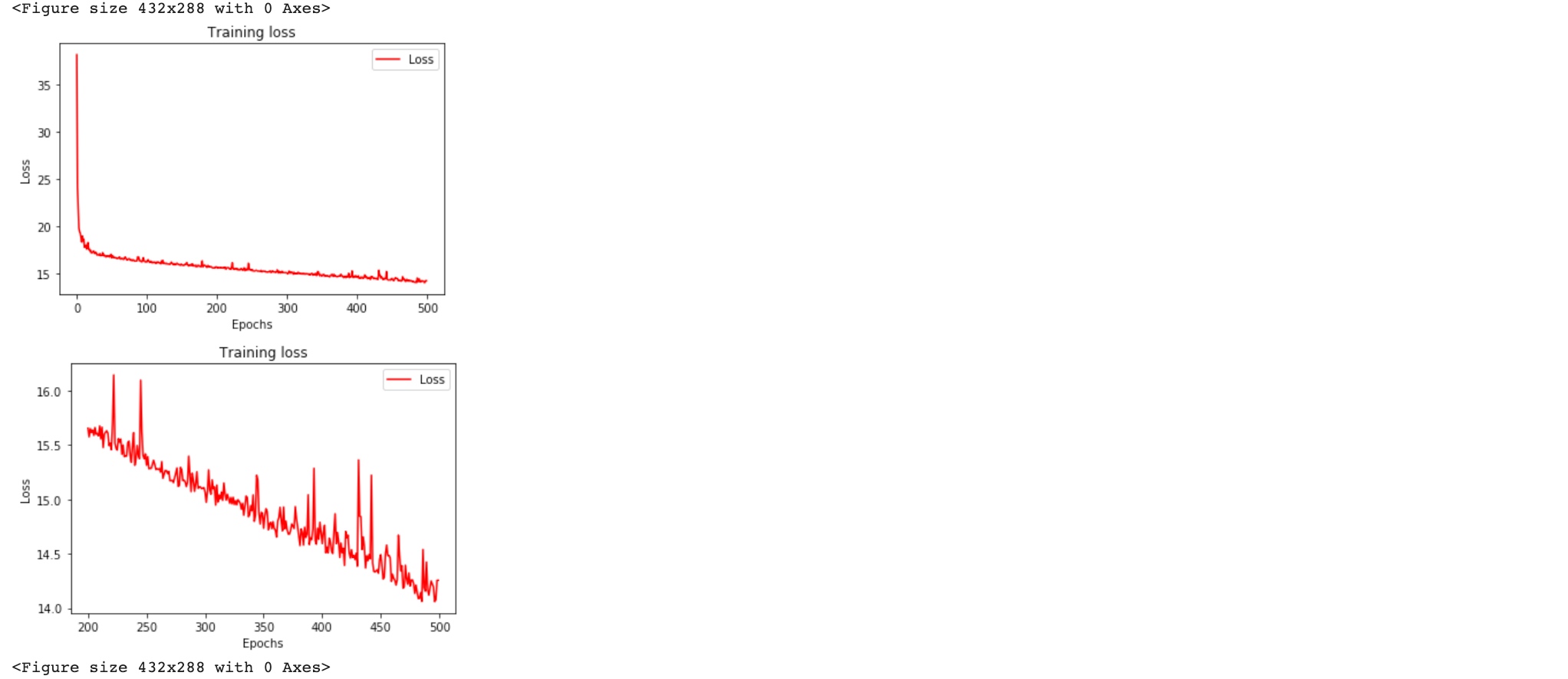
plt.plot(epochs, loss, 'r')
plt.title('Training loss')
plt.xlabel("Epochs")
plt.ylabel("Loss")
plt.legend(["Loss"])

plt.figure()



zoomed_loss = loss[200:]
zoomed_epochs = range(200,500)


#------------------------------------------------
# Plot training and validation loss per epoch
#------------------------------------------------
plt.plot(zoomed_epochs, zoomed_loss, 'r')
plt.title('Training loss')
plt.xlabel("Epochs")
plt.ylabel("Loss")
plt.legend(["Loss"])

plt.figure()


print(rnn_forecast)
# [128.34058   117.36959   120.21221   132.9964    119.64408   152.58786
#  181.13803   185.29076   173.63475   132.6062    150.20526   160.88815
#  163.61447   171.61197   211.39217   221.32239   224.66443   214.8448
#  191.54178   192.60901   189.11853   191.98352   214.38405   212.87851
#  166.91495   156.36555   155.82523   178.84999   175.02908   140.73271
#  196.68854   131.36443   126.95976   204.3727    150.5691    162.80179
#  174.71324   140.41599   139.38342   147.95525   176.58795   175.7258
#  165.33727   162.73628   193.00378   171.122     171.76006   161.18188
#  162.52214   134.54166   109.517654  123.663284  112.04064   109.65196
#  113.83678   112.192474  103.10232    97.70291    94.381096   77.466324
#   71.36468    66.25992    70.35916    69.88442    61.27887    61.12542
#   62.034565   70.3916     68.30441    58.10794    59.131485   63.385876
#   51.6235     46.63688    45.235954   45.366383   39.75632    53.87586
#   41.329395   40.827908   42.400898   30.238804   24.05354    24.577883
#   38.752895   21.109665   18.151054   13.467979   23.478064   12.376457
#   24.793894   28.246105   26.681725   21.532541   13.384017   16.750313
#   14.127593   15.409324   12.572709   10.20132     9.147289    9.518226
#   11.346884    9.0025215  10.529169    8.679348    8.762336   10.009352
#   11.721095    4.1075974   3.9611936  10.6716585  10.2986765  10.185544
#    8.890774   10.894372    7.550009    4.496826    5.534169    6.7954316
#    5.8580966   4.6634855   3.813833    3.1663089   1.9660205   2.045089
#    3.404832    4.248945    3.2749965   4.0231943   5.004154    5.804768
#    9.53496    12.965054   23.986254   28.201658   29.027748   34.14526
#   30.276499   23.797646   31.94648    41.194927   48.054516   59.91797
#   58.944393   55.677586   57.871212   69.41632    78.50339    74.4383
#   76.275185   79.53018    85.66454   102.888504  100.1326    107.128265
#  117.89254    99.49634    64.943375   87.370804  101.40014    97.493484
#  107.98509   105.63581    98.854294   95.5105     85.1918     84.97572
#   73.87473    87.63814    90.77395    88.48726    99.78565    97.055016
#   89.09171    78.62403    78.823      67.49795   105.22152    90.97482
#   93.25439   112.44844   126.05207   113.95221   103.48979   110.45583
#   95.54847    92.05747    96.47111   112.35267    97.895386   92.47728
#  117.28922    99.902435  100.44479    80.723854   81.158844   91.761375
#   81.511314   78.516304   75.57877    78.155014   69.66825    63.55747
#   61.498325   58.756805   54.520493   53.019154   46.919525   46.18231
#   37.52933    39.278973   35.69973    30.163843   27.670712   31.556252
#   27.721      21.709484   22.650421   14.038152   20.04164    17.108953
#   15.086285   15.668817   16.351469   19.145948   12.436576   11.963836
#   10.746365    9.13576     8.551076    5.63045     7.8610287   8.263008
#    9.631194 ]

-w1022