2. Convolutional Neural Networks in TensorFlow
Exploring a larger dataset
Use Tensorflow 2.x in colab
%tensorflow_version 2.x

import tensorflow as tf
print(tf.__version__)
The 2,000 images used in this exercise are excerpted from the “Dogs vs. Cats” dataset available on Kaggle, which contains 25,000 images
Load Data:
# Get 2000 images
!wget --no-check-certificate \
https://storage.googleapis.com/mledu-datasets/cats_and_dogs_filtered.zip \
-O /tmp/cats_and_dogs_filtered.zip

import os
import zipfile

local_zip = '/tmp/cats_and_dogs_filtered.zip'

zip_ref = zipfile.ZipFile(local_zip, 'r')

zip_ref.extractall('/tmp')
zip_ref.close()

# ----------------

base_dir = '/tmp/cats_and_dogs_filtered'

train_dir = os.path.join(base_dir, 'train')
validation_dir = os.path.join(base_dir, 'validation')

# Directory with our training cat/dog pictures
train_cats_dir = os.path.join(train_dir, 'cats')
train_dogs_dir = os.path.join(train_dir, 'dogs')

# Directory with our validation cat/dog pictures
validation_cats_dir = os.path.join(validation_dir, 'cats')
validation_dogs_dir = os.path.join(validation_dir, 'dogs')

# ----------------

train_cat_fnames = os.listdir( train_cats_dir )
train_dog_fnames = os.listdir( train_dogs_dir )

print(train_cat_fnames[:10])  # ['cat.152.jpg', 'cat.72.jpg', 'cat.118.jpg', ....]
print(train_dog_fnames[:10])  # ['dog.909.jpg', 'dog.654.jpg', 'dog.960.jpg', ...]

# ----------------

print('total training cat images :', len(os.listdir(      train_cats_dir ) ))  # total training cat images : 1000
print('total training dog images :', len(os.listdir(      train_dogs_dir ) )) # total training dog images : 1000

print('total validation cat images :', len(os.listdir( validation_cats_dir ) )) # total validation cat images : 500
print('total validation dog images :', len(os.listdir( validation_dogs_dir ) ))  # total validation dog images : 500
Data Visualization:
%matplotlib inline

import matplotlib.image as mpimg
import matplotlib.pyplot as plt

# Parameters for our graph; we'll output images in a 4x4 configuration
nrows = 4
ncols = 4

pic_index = 0 # Index for iterating over images

# ---------------

# Set up matplotlib fig, and size it to fit 4x4 pics
fig = plt.gcf()
fig.set_size_inches(ncols*4, nrows*4)

pic_index+=8

next_cat_pix = [os.path.join(train_cats_dir, fname)
            for fname in train_cat_fnames[ pic_index-8:pic_index]
           ]

next_dog_pix = [os.path.join(train_dogs_dir, fname)
            for fname in train_dog_fnames[ pic_index-8:pic_index]
           ]

for i, img_path in enumerate(next_cat_pix+next_dog_pix):
# Set up subplot; subplot indices start at 1
sp = plt.subplot(nrows, ncols, i + 1)
sp.axis('Off') # Don't show axes (or gridlines)

img = mpimg.imread(img_path)
plt.imshow(img)

plt.show()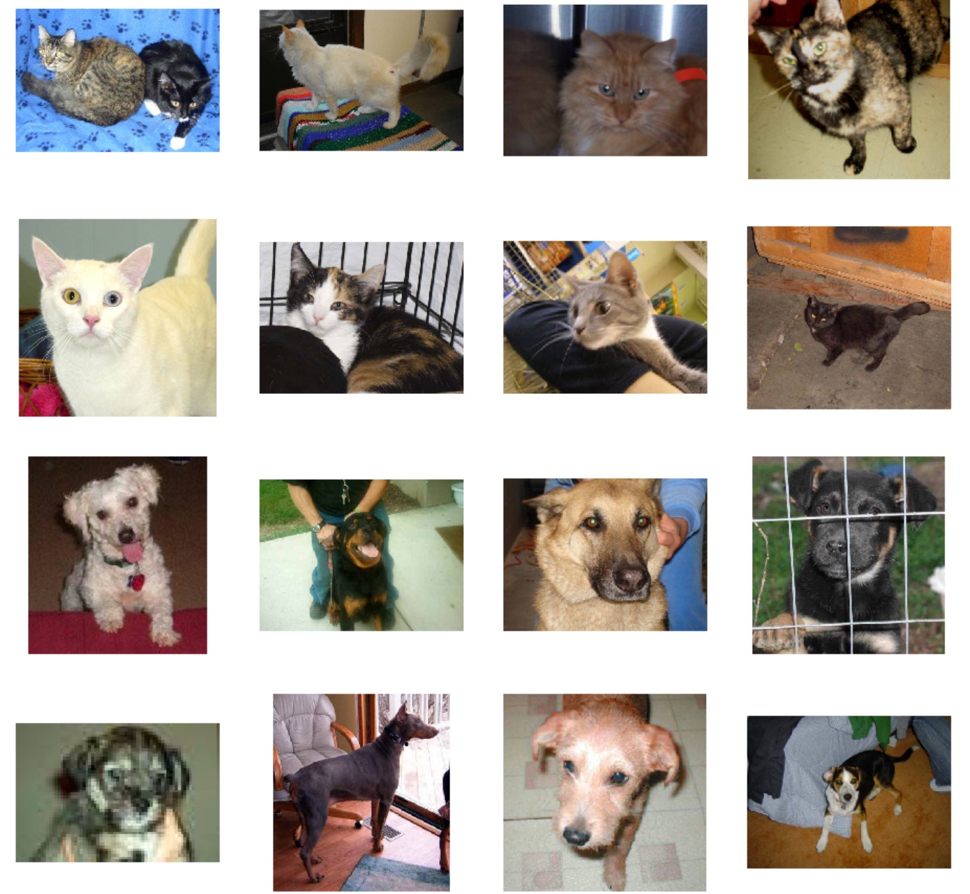
Build Model:
import tensorflow as tf

model = tf.keras.models.Sequential([
# Note the input shape is the desired size of the image 150x150 with 3 bytes color
tf.keras.layers.Conv2D(16, (3,3), activation='relu', input_shape=(150, 150, 3)),
tf.keras.layers.MaxPooling2D(2,2),
tf.keras.layers.Conv2D(32, (3,3), activation='relu'),
tf.keras.layers.MaxPooling2D(2,2),
tf.keras.layers.Conv2D(64, (3,3), activation='relu'),
tf.keras.layers.MaxPooling2D(2,2),
# Flatten the results to feed into a DNN
tf.keras.layers.Flatten(),
# 512 neuron hidden layer
tf.keras.layers.Dense(512, activation='relu'),
# Only 1 output neuron. It will contain a value from 0-1 where 0 for 1 class ('cats') and 1 for the other ('dogs')
tf.keras.layers.Dense(1, activation='sigmoid')
])

model.summary()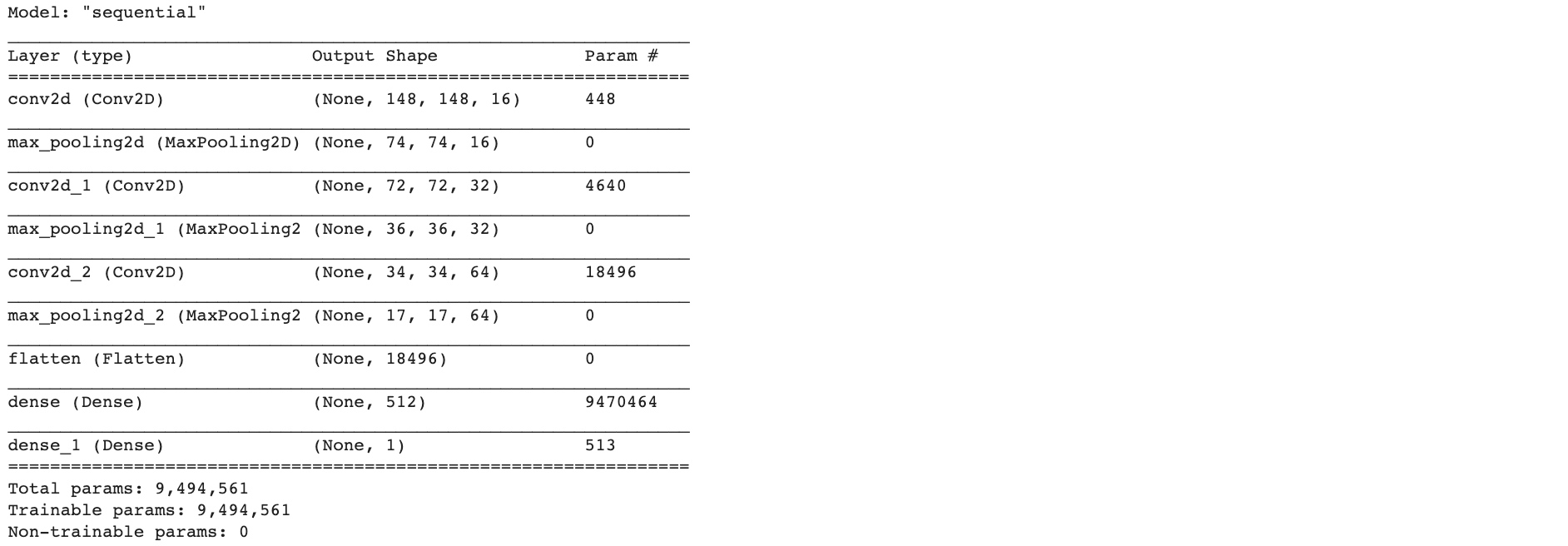
Configure the specifications for model training:
from tensorflow.keras.optimizers import RMSprop

model.compile(optimizer=RMSprop(lr=0.001),
          loss='binary_crossentropy',
          metrics = ['acc'])
Data Preprocessing:
from tensorflow.keras.preprocessing.image import ImageDataGenerator

# All images will be rescaled by 1./255.
train_datagen = ImageDataGenerator( rescale = 1.0/255. )
test_datagen  = ImageDataGenerator( rescale = 1.0/255. )

# --------------------
# Flow training images in batches of 20 using train_datagen generator
# --------------------
train_generator = train_datagen.flow_from_directory(train_dir,
                                                batch_size=20,
                                                class_mode='binary',
                                                target_size=(150, 150))
# --------------------
# Flow validation images in batches of 20 using test_datagen generator
# --------------------
validation_generator =  test_datagen.flow_from_directory(validation_dir,
                                                     batch_size=20,
                                                     class_mode  = 'binary',
                                                     target_size = (150, 150))
Training:
history = model.fit_generator(train_generator,
                          validation_data=validation_generator,
                          steps_per_epoch=100,
                          epochs=15,
                          validation_steps=50,
                          verbose=2)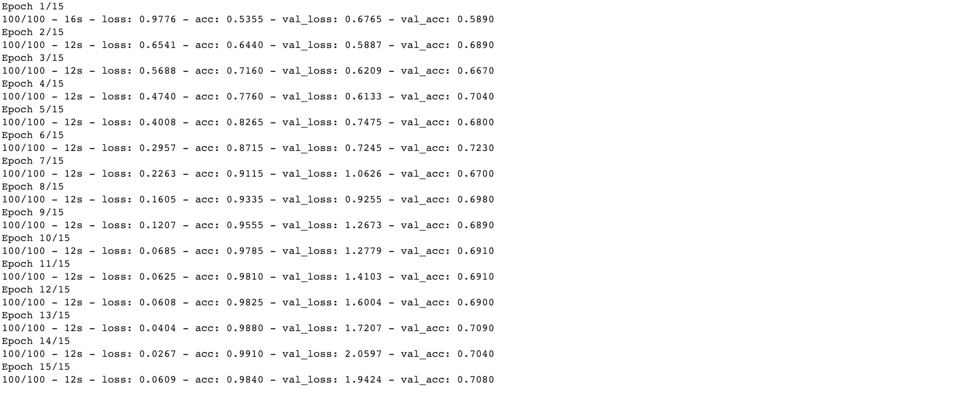
see 4 values per epoch – Loss, Accuracy, Validation Loss and Validation Accuracy.
Run the model:
import numpy as np

from google.colab import files
from keras.preprocessing import image

uploaded=files.upload()

for fn in uploaded.keys():

# predicting images
path='/content/' + fn
img=image.load_img(path, target_size=(150, 150))

x=image.img_to_array(img)
x=np.expand_dims(x, axis=0)
images = np.vstack([x])

classes = model.predict(images, batch_size=10)

print(classes[0])

if classes[0]>0:
print(fn + " is a dog")

else:
print(fn + " is a cat")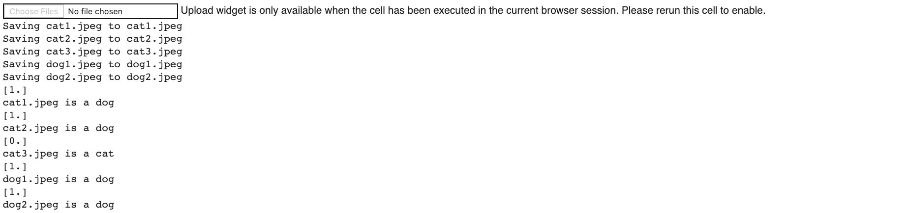
Visualize Intermediate Representations:
import numpy as np
import random
from   tensorflow.keras.preprocessing.image import img_to_array, load_img

# Let's define a new Model that will take an image as input, and will output
# intermediate representations for all layers in the previous model after
# the first.
successive_outputs = [layer.output for layer in model.layers[1:]]

#visualization_model = Model(img_input, successive_outputs)
visualization_model = tf.keras.models.Model(inputs = model.input, outputs = successive_outputs)

# Let's prepare a random input image of a cat or dog from the training set.
cat_img_files = [os.path.join(train_cats_dir, f) for f in train_cat_fnames]
dog_img_files = [os.path.join(train_dogs_dir, f) for f in train_dog_fnames]

img_path = random.choice(cat_img_files + dog_img_files)
img = load_img(img_path, target_size=(150, 150))  # this is a PIL image

x   = img_to_array(img)                           # Numpy array with shape (150, 150, 3)
x   = x.reshape((1,) + x.shape)                   # Numpy array with shape (1, 150, 150, 3)

# Rescale by 1/255
x /= 255.0

# Let's run our image through our network, thus obtaining all
# intermediate representations for this image.
successive_feature_maps = visualization_model.predict(x)

# These are the names of the layers, so can have them as part of our plot
layer_names = [layer.name for layer in model.layers]

# -----------------------------------------------------------------------
# Now let's display our representations
# -----------------------------------------------------------------------
for layer_name, feature_map in zip(layer_names, successive_feature_maps):

if len(feature_map.shape) == 4:

#-------------------------------------------
# Just do this for the conv / maxpool layers, not the fully-connected layers
#-------------------------------------------
n_features = feature_map.shape[-1]  # number of features in the feature map
size       = feature_map.shape[ 1]  # feature map shape (1, size, size, n_features)

# We will tile our images in this matrix
display_grid = np.zeros((size, size * n_features))

#-------------------------------------------------
# Postprocess the feature to be visually palatable
#-------------------------------------------------
for i in range(n_features):
  x  = feature_map[0, :, :, i]
  x -= x.mean()
  x /= x.std ()
  x *=  64
  x += 128
  x  = np.clip(x, 0, 255).astype('uint8')
  display_grid[:, i * size : (i + 1) * size] = x # Tile each filter into a horizontal grid

#-----------------
# Display the grid
#-----------------

scale = 20. / n_features
plt.figure( figsize=(scale * n_features, scale) )
plt.title ( layer_name )
plt.grid  ( False )
plt.imshow( display_grid, aspect='auto', cmap='viridis' )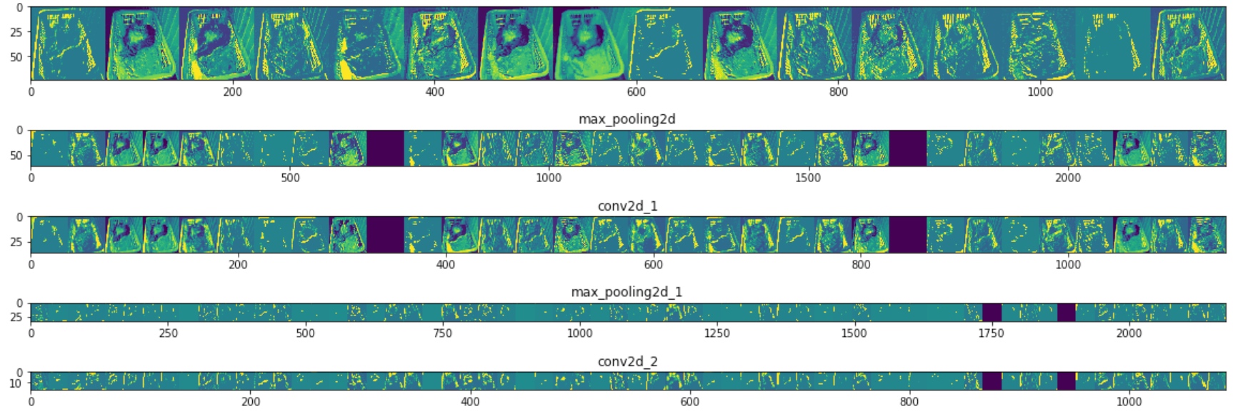
Evaluating Accuracy and Loss for the Model:
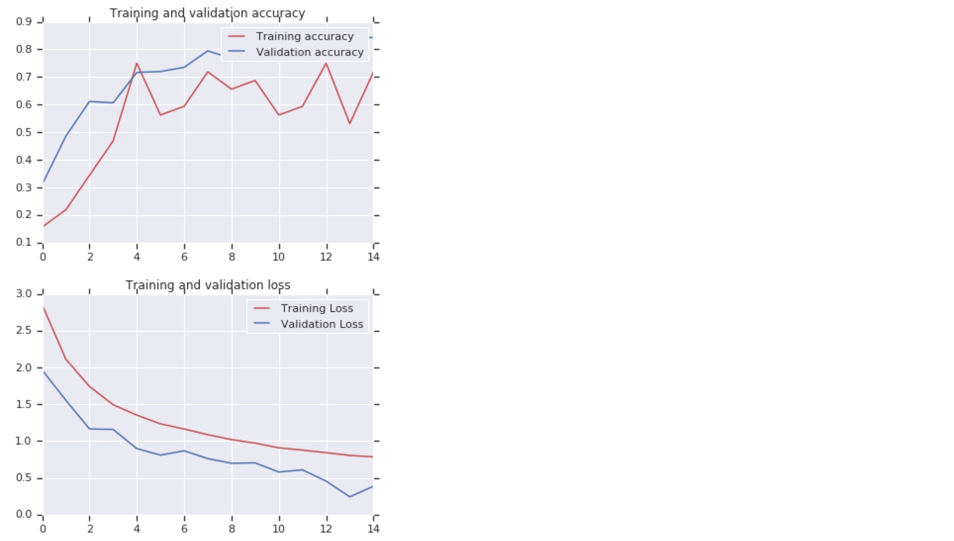
#-----------------------------------------------------------
# Retrieve a list of list results on training and test data
# sets for each training epoch
#-----------------------------------------------------------
acc      = history.history[     'acc' ]
val_acc  = history.history[ 'val_acc' ]
loss     = history.history[    'loss' ]
val_loss = history.history['val_loss' ]

epochs   = range(len(acc)) # Get number of epochs

#------------------------------------------------
# Plot training and validation accuracy per epoch
#------------------------------------------------
plt.plot  ( epochs,     acc )
plt.plot  ( epochs, val_acc )
plt.title ('Training and validation accuracy')
plt.figure()

#------------------------------------------------
# Plot training and validation loss per epoch
#------------------------------------------------
plt.plot  ( epochs,     loss )
plt.plot  ( epochs, val_loss )
plt.title ('Training and validation loss'   )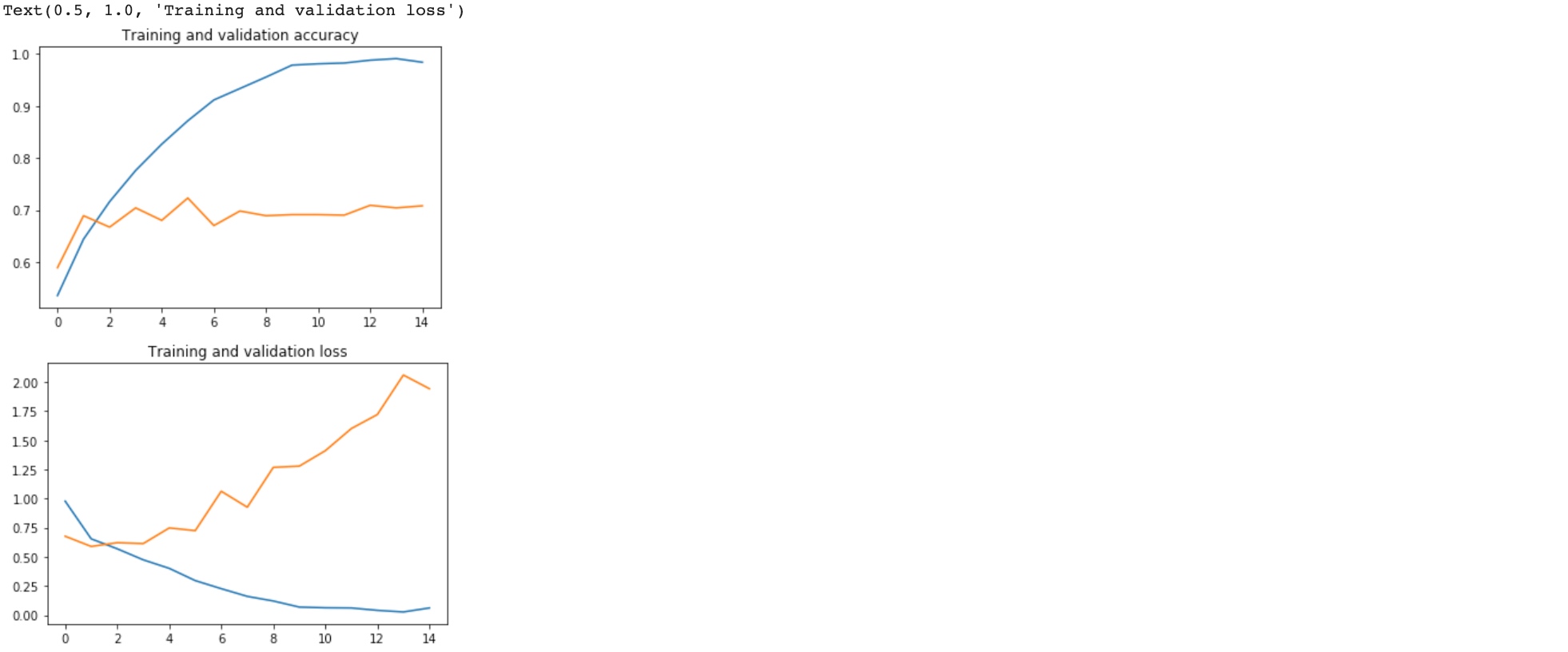
It is overfitting. (High performance in training set and poor performance in validation set). After 2 epochs, the accuracy of validation set is barely changed.
Clean up - terminate the kernel and free memory resources:
import os, signal
os.kill(os.getpid(), signal.SIGKILL)
Augmentation - a technique to avoid overfitting
Augmentation simply amends your images on-the-fly while training using transforms like rotation. So, it could ‘simulate’ an image of a cat lying down by rotating a ‘standing’ cat by 90 degrees. As such you get a cheap way of extending your dataset beyond what you have already.
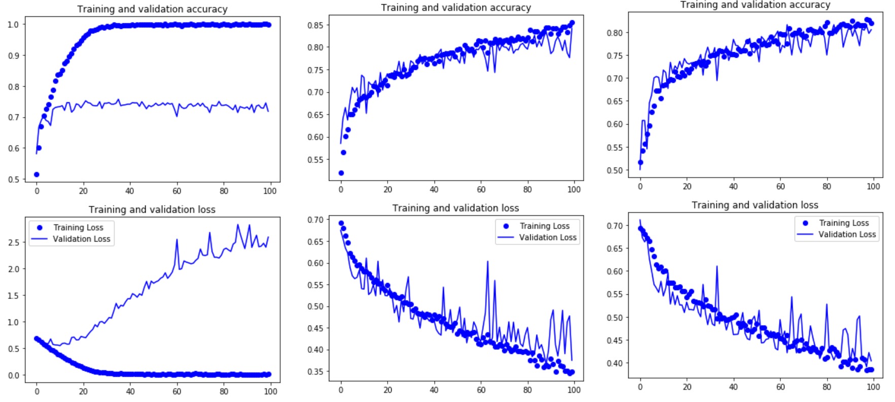
‘Cats V.S. Dogs’ mdoel performance from left to right:
- Without Image Augmentation
- With Image Augmentation
- With Augmentation & Dropout
Code(With Augmentation & Dropout):
!wget --no-check-certificate \
    https://storage.googleapis.com/mledu-datasets/cats_and_dogs_filtered.zip \
    -O /tmp/cats_and_dogs_filtered.zip

import os
import zipfile
import tensorflow as tf
from tensorflow.keras.optimizers import RMSprop
from tensorflow.keras.preprocessing.image import ImageDataGenerator

local_zip = '/tmp/cats_and_dogs_filtered.zip'
zip_ref = zipfile.ZipFile(local_zip, 'r')
zip_ref.extractall('/tmp')
zip_ref.close()

base_dir = '/tmp/cats_and_dogs_filtered'
train_dir = os.path.join(base_dir, 'train')
validation_dir = os.path.join(base_dir, 'validation')

# Directory with our training cat pictures
train_cats_dir = os.path.join(train_dir, 'cats')

# Directory with our training dog pictures
train_dogs_dir = os.path.join(train_dir, 'dogs')

# Directory with our validation cat pictures
validation_cats_dir = os.path.join(validation_dir, 'cats')

# Directory with our validation dog pictures
validation_dogs_dir = os.path.join(validation_dir, 'dogs')

model = tf.keras.models.Sequential([
    tf.keras.layers.Conv2D(32, (3,3), activation='relu', input_shape=(150, 150, 3)),
    tf.keras.layers.MaxPooling2D(2, 2),
    tf.keras.layers.Conv2D(64, (3,3), activation='relu'),
    tf.keras.layers.MaxPooling2D(2,2),
    tf.keras.layers.Conv2D(128, (3,3), activation='relu'),
    tf.keras.layers.MaxPooling2D(2,2),
    tf.keras.layers.Conv2D(128, (3,3), activation='relu'),
    tf.keras.layers.MaxPooling2D(2,2),
    tf.keras.layers.Dropout(0.5), #!!!!!!!!!!!!!!!!!!!!!!!!!!!!!!!!!!!!!!!!!!Dropout
    tf.keras.layers.Flatten(),
    tf.keras.layers.Dense(512, activation='relu'),
    tf.keras.layers.Dense(1, activation='sigmoid')
])

model.compile(loss='binary_crossentropy',
              optimizer=RMSprop(lr=1e-4),
              metrics=['acc'])

# This code has changed. Now instead of the ImageGenerator just rescaling
# the image, we also rotate and do other operations
# Updated to do image augmentation
train_datagen = ImageDataGenerator(
      rescale=1./255,
      rotation_range=40,
      width_shift_range=0.2,
      height_shift_range=0.2,
      shear_range=0.2,
      zoom_range=0.2,
      horizontal_flip=True,
      fill_mode='nearest')

test_datagen = ImageDataGenerator(rescale=1./255)

# Flow training images in batches of 20 using train_datagen generator
train_generator = train_datagen.flow_from_directory(
        train_dir,  # This is the source directory for training images
        target_size=(150, 150),  # All images will be resized to 150x150
        batch_size=20,
        # Since we use binary_crossentropy loss, we need binary labels
        class_mode='binary')

# Flow validation images in batches of 20 using test_datagen generator
validation_generator = test_datagen.flow_from_directory(
        validation_dir,
        target_size=(150, 150),
        batch_size=20,
        class_mode='binary')

history = model.fit_generator(
      train_generator,
      steps_per_epoch=100,  # 2000 images = batch_size * steps
      epochs=100,
      validation_data=validation_generator,
      validation_steps=50,  # 1000 images = batch_size * steps
      verbose=2)
Exercise:
%tensorflow_version 2.x

import os
import zipfile
import random
import tensorflow as tf
from tensorflow.keras.optimizers import RMSprop
from tensorflow.keras.preprocessing.image import ImageDataGenerator
from shutil import copyfile

tf.__version__
!wget --no-check-certificate \
"https://download.microsoft.com/download/3/E/1/3E1C3F21-ECDB-4869-8368-6DEBA77B919F/kagglecatsanddogs_3367a.zip" \
-O "/tmp/cats-and-dogs.zip"
local_zip = '/tmp/cats-and-dogs.zip'
zip_ref = zipfile.ZipFile(local_zip, 'r')
zip_ref.extractall('/tmp')
zip_ref.close()
print(len(os.listdir('/tmp/PetImages/Cat/'))) # 12501
print(len(os.listdir('/tmp/PetImages/Dog/'))) # 12501try:
os.mkdir('/tmp/cats-v-dogs')
os.mkdir('/tmp/cats-v-dogs/training')
os.mkdir('/tmp/cats-v-dogs/testing')
os.mkdir('/tmp/cats-v-dogs/training/cats')
os.mkdir('/tmp/cats-v-dogs/training/dogs')
os.mkdir('/tmp/cats-v-dogs/testing/cats')
os.mkdir('/tmp/cats-v-dogs/testing/dogs')
except OSError:
passdef split_data(SOURCE, TRAINING, TESTING, SPLIT_SIZE):
files = []
for filename in os.listdir(SOURCE):
file = SOURCE + filename
if os.path.getsize(file) > 0:
files.append(filename)
else:
print(filename + " is zero length, so ignoring.")
training_length = int(len(files) * SPLIT_SIZE)
testing_length = int(len(files) - training_length)
shuffled_set = random.sample(files, len(files))
training_set = shuffled_set[0:training_length]
testing_set = shuffled_set[:testing_length]
for filename in training_set:
this_file = SOURCE + filename
destination = TRAINING + filename
copyfile(this_file, destination)
for filename in testing_set:
this_file = SOURCE + filename
destination = TESTING + filename
copyfile(this_file, destination)
CAT_SOURCE_DIR = "/tmp/PetImages/Cat/"
TRAINING_CATS_DIR = "/tmp/cats-v-dogs/training/cats/"
TESTING_CATS_DIR = "/tmp/cats-v-dogs/testing/cats/"
DOG_SOURCE_DIR = "/tmp/PetImages/Dog/"
TRAINING_DOGS_DIR = "/tmp/cats-v-dogs/training/dogs/"
TESTING_DOGS_DIR = "/tmp/cats-v-dogs/testing/dogs/"
split_size = .9
split_data(CAT_SOURCE_DIR, TRAINING_CATS_DIR, TESTING_CATS_DIR, split_size)
split_data(DOG_SOURCE_DIR, TRAINING_DOGS_DIR, TESTING_DOGS_DIR, split_size)
# Expected output
# 666.jpg is zero length, so ignoring
# 11702.jpg is zero length, so ignoringprint(len(os.listdir('/tmp/cats-v-dogs/training/cats/')))
print(len(os.listdir('/tmp/cats-v-dogs/training/dogs/')))
print(len(os.listdir('/tmp/cats-v-dogs/testing/cats/')))
print(len(os.listdir('/tmp/cats-v-dogs/testing/dogs/')))
# Expected output:
# 11250
# 11250
# 1250
# 1250model = tf.keras.models.Sequential([
tf.keras.layers.Conv2D(16, (3, 3), activation='relu', input_shape=(150, 150, 3)),
tf.keras.layers.MaxPooling2D(2, 2),
tf.keras.layers.Conv2D(32, (3, 3), activation='relu'),
tf.keras.layers.MaxPooling2D(2, 2),
tf.keras.layers.Conv2D(64, (3, 3), activation='relu'),
tf.keras.layers.MaxPooling2D(2, 2),
tf.keras.layers.Flatten(),
tf.keras.layers.Dense(512, activation='relu'),
tf.keras.layers.Dense(1, activation='sigmoid')
])
model.compile(optimizer=RMSprop(lr=0.001), loss='binary_crossentropy', metrics=['acc'])Image Augmentation:
- rotation_range is a value in degrees (0–180), a range within which to randomly rotate pictures.
- width_shift and height_shift are ranges (as a fraction of total width or height) within which to randomly translate pictures vertically or horizontally.
- shear_range is for randomly applying shearing transformations.
- zoom_range is for randomly zooming inside pictures.
- horizontal_flip is for randomly flipping half of the images horizontally. This is relevant when there are no assumptions of horizontal assymmetry (e.g. real-world pictures).
- fill_mode is the strategy used for filling in newly created pixels, which can appear after a rotation or a width/height shift.
code:
TRAINING_DIR = "/tmp/cats-v-dogs/training/"
train_datagen = ImageDataGenerator(rescale=1./255,
      rotation_range=40,
      width_shift_range=0.2,
      height_shift_range=0.2,
      shear_range=0.2,
      zoom_range=0.2,
      horizontal_flip=True,
      fill_mode='nearest')
train_generator = train_datagen.flow_from_directory(TRAINING_DIR,
                                                    batch_size=100,
                                                    class_mode='binary',
                                                    target_size=(150, 150))

VALIDATION_DIR = "/tmp/cats-v-dogs/testing/"
# Experiment with your own parameters here to really try to drive it to 99.9% accuracy or better
validation_datagen = ImageDataGenerator(rescale=1./255)
validation_generator = validation_datagen.flow_from_directory(VALIDATION_DIR,
                                                              batch_size=100,
                                                              class_mode='binary',
                                                              target_size=(150, 150))

# Expected Output:
# Found 22498 images belonging to 2 classes.
# Found 2500 images belonging to 2 classes.
Noted that: Validation Set should not be augmented, otherwise, the plot of accuracy and loss graph is so fluctuant and the performance is not good as well.
# Define a Callback class that stops training once accuracy reaches 95.9%
class myCallback(tf.keras.callbacks.Callback):
  def on_epoch_end(self, epoch, logs={}):
    if(logs.get('acc')>0.959):
      print("\nReached 95.9% accuracy so cancelling training!")
      self.model.stop_training = True

callbacks = myCallback()

history = model.fit_generator(train_generator,
                              epochs=15,
                              verbose=1,
                              validation_data=validation_generator
                              callbacks=[callbacks]
                              )
%matplotlib inline

import matplotlib.image  as mpimg
import matplotlib.pyplot as plt

#-----------------------------------------------------------
# Retrieve a list of list results on training and test data
# sets for each training epoch
#-----------------------------------------------------------
acc=history.history['acc']
val_acc=history.history['val_acc']
loss=history.history['loss']
val_loss=history.history['val_loss']

epochs=range(len(acc)) # Get number of epochs

#------------------------------------------------
# Plot training and validation accuracy per epoch
#------------------------------------------------
plt.plot(epochs, acc, 'r', "Training Accuracy")
plt.plot(epochs, val_acc, 'b', "Validation Accuracy")
plt.title('Training and validation accuracy')
plt.figure()

#------------------------------------------------
# Plot training and validation loss per epoch
#------------------------------------------------
plt.plot(epochs, loss, 'r', "Training Loss")
plt.plot(epochs, val_loss, 'b', "Validation Loss")
plt.figure()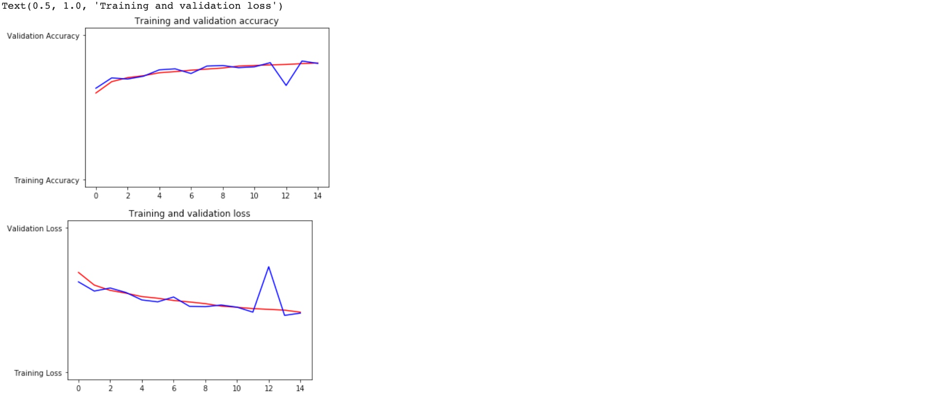
import numpy as np
from google.colab import files
from keras.preprocessing import image

uploaded = files.upload()

for fn in uploaded.keys():

  # predicting images
  path = '/content/' + fn
  img = image.load_img(path, target_size=(150, 150))
  x = image.img_to_array(img)
  x = np.expand_dims(x, axis=0)

  images = np.vstack([x])
  classes = model.predict(images, batch_size=10)
  print(classes[0])
  if classes[0]>0.5:
    print(fn + " is a dog")
  else:
    print(fn + " is a cat")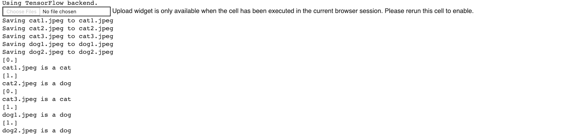
Transfer Learning
- use the keras layers API to pick at the layers
- download the snapshot of the model from the URL which saved a copy of pretained weight
- use the keras inception_v3 API for Inception model definition. Instantiate that with the desired input shape
- set ‘include_top’ to false to ignore the fully-connected layer at the top
- iterate through its layers and lock them (not trainable with this code)
- the bottom layer is ‘mixed10’ which convoluted to 3 by 3. (examine by
model.summary) - Can set the ‘last_layer’ to ‘mixed7’ which convoluted 7 by 7 (via
model.get_layer('mixed7')) and take the output from it (‘last_output’) as the input InceptionV3 model
code:
%tensorflow_version 2.x
import os

from tensorflow.keras import layers
from tensorflow.keras import Model

# A copy of the pretrained weights for the inception neural network is saved at this URL
!wget --no-check-certificate \
    https://storage.googleapis.com/mledu-datasets/inception_v3_weights_tf_dim_ordering_tf_kernels_notop.h5 \
    -O /tmp/inception_v3_weights_tf_dim_ordering_tf_kernels_notop.h5

from tensorflow.keras.applications.inception_v3 import InceptionV3

local_weights_file = '/tmp/inception_v3_weights_tf_dim_ordering_tf_kernels_notop.h5'

pre_trained_model = InceptionV3(input_shape = (150, 150, 3),
                                include_top = False,
                                weights = None)

pre_trained_model.load_weights(local_weights_file)

for layer in pre_trained_model.layers:
    layer.trainable = False

pre_trained_model.summary()

last_layer = pre_trained_model.get_layer('mixed7')
print('last layer output shape: ', last_layer.output_shape)
last_output = last_layer.output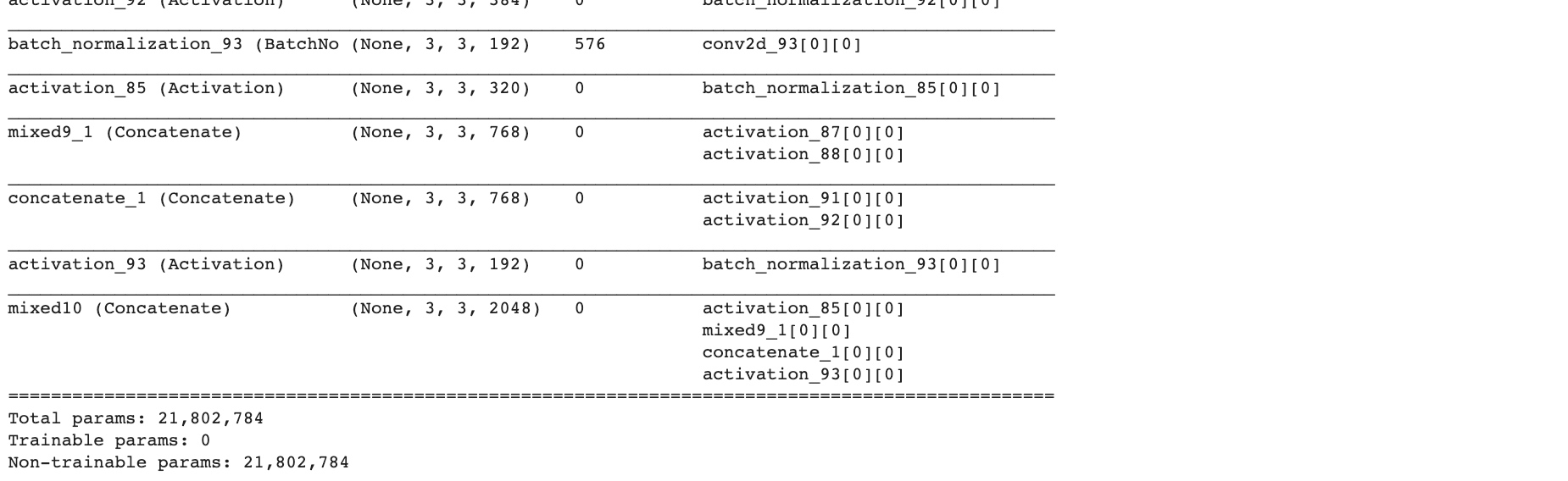
Regularization using dropouts to make your network more efficient in preventing over-specialization and overfitting. The idea behind Dropouts is that they remove a random number of neurons in your neural network.
This works very well for two reasons:
- neighboring neurons often end up with similar weights, which can lead to overfitting, so dropping some out at random can remove this.
- often a neuron can over-weigh the input from a neuron in the previous layer, and can over specialize as a result.
Add own DNN underneath ‘mixed7’ so that you could retrain on images using the convolutions from the other model:
from tensorflow.keras.optimizers import RMSprop

# Flatten the output layer to 1 dimension
x = layers.Flatten()(last_output)
# Add a fully connected layer with 1,024 hidden units and ReLU activation
x = layers.Dense(1024, activation='relu')(x)
# Add a dropout rate of 0.2
x = layers.Dropout(0.2)(x)
# Add a final sigmoid layer for classification
x = layers.Dense  (1, activation='sigmoid')(x)

model = Model( pre_trained_model.input, x)

model.compile(optimizer = RMSprop(lr=0.0001),
              loss = 'binary_crossentropy',
              metrics = ['acc'])

model.summary()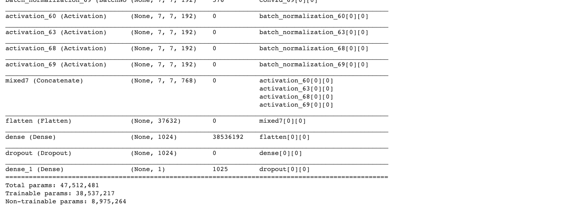
!wget --no-check-certificate \
        https://storage.googleapis.com/mledu-datasets/cats_and_dogs_filtered.zip \
       -O /tmp/cats_and_dogs_filtered.zip

from tensorflow.keras.preprocessing.image import ImageDataGenerator

import os
import zipfile

local_zip = '//tmp/cats_and_dogs_filtered.zip'

zip_ref = zipfile.ZipFile(local_zip, 'r')

zip_ref.extractall('/tmp')
zip_ref.close()

# Define our example directories and files
base_dir = '/tmp/cats_and_dogs_filtered'

train_dir = os.path.join( base_dir, 'train')
validation_dir = os.path.join( base_dir, 'validation')


train_cats_dir = os.path.join(train_dir, 'cats') # Directory with our training cat pictures
train_dogs_dir = os.path.join(train_dir, 'dogs') # Directory with our training dog pictures
validation_cats_dir = os.path.join(validation_dir, 'cats') # Directory with our validation cat pictures
validation_dogs_dir = os.path.join(validation_dir, 'dogs')# Directory with our validation dog pictures

train_cat_fnames = os.listdir(train_cats_dir)
train_dog_fnames = os.listdir(train_dogs_dir)

# Add our data-augmentation parameters to ImageDataGenerator
train_datagen = ImageDataGenerator(rescale = 1./255.,
                                   rotation_range = 40,
                                   width_shift_range = 0.2,
                                   height_shift_range = 0.2,
                                   shear_range = 0.2,
                                   zoom_range = 0.2,
                                   horizontal_flip = True)

# Note that the validation data should not be augmented!
test_datagen = ImageDataGenerator( rescale = 1.0/255. )

# Flow training images in batches of 20 using train_datagen generator
train_generator = train_datagen.flow_from_directory(train_dir,
                                                    batch_size = 20,
                                                    class_mode = 'binary',
                                                    target_size = (150, 150))

# Flow validation images in batches of 20 using test_datagen generator
validation_generator =  test_datagen.flow_from_directory( validation_dir,
                                                          batch_size  = 20,
                                                          class_mode  = 'binary',
                                                          target_size = (150, 150))
history = model.fit_generator(
train_generator,
validation_data = validation_generator,
steps_per_epoch = 100,
epochs = 20,
validation_steps = 50,
verbose = 2)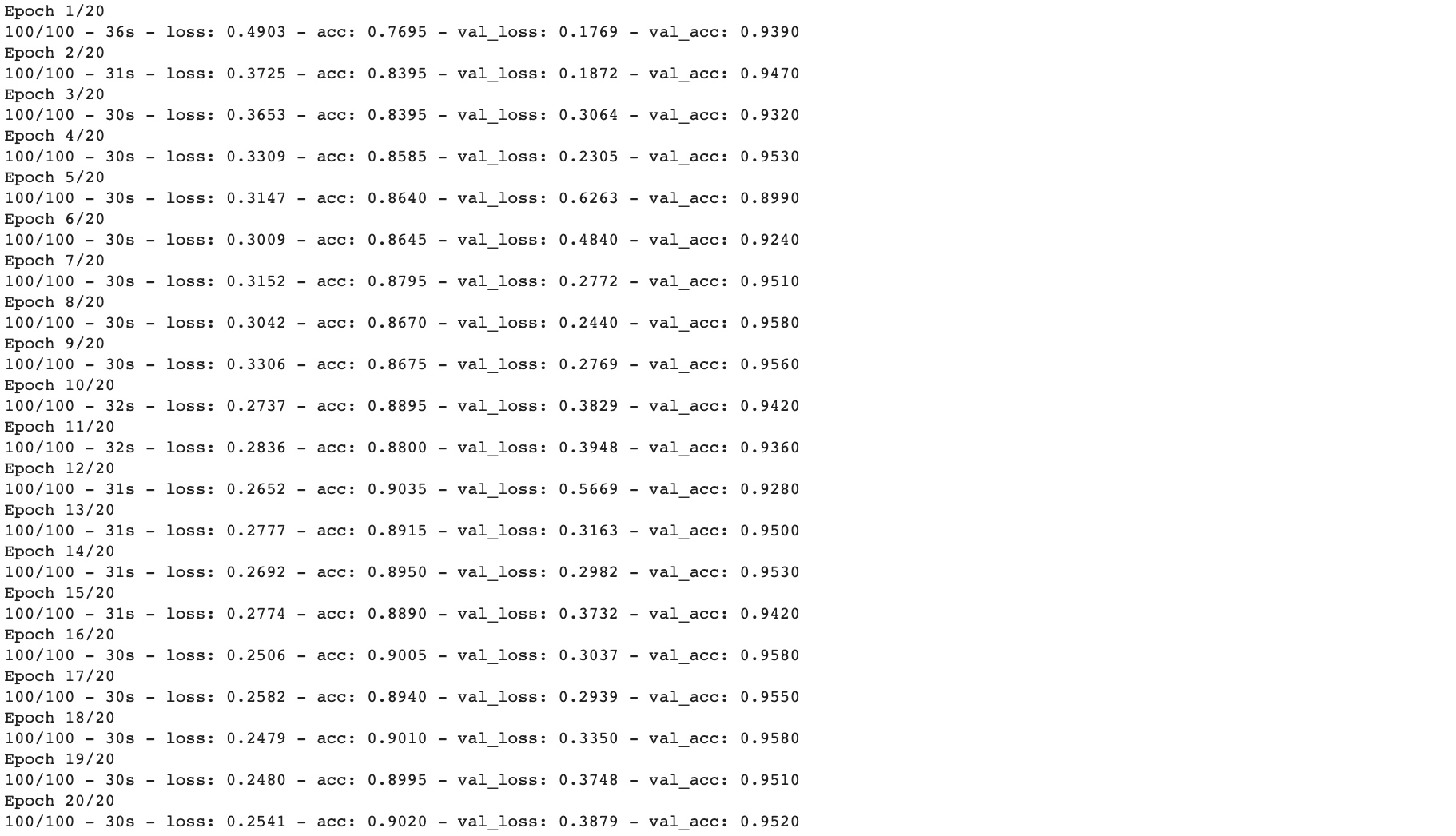
import matplotlib.pyplot as plt
acc = history.history['acc']
val_acc = history.history['val_acc']
loss = history.history['loss']
val_loss = history.history['val_loss']

epochs = range(len(acc))

plt.plot(epochs, acc, 'r', label='Training accuracy')
plt.plot(epochs, val_acc, 'b', label='Validation accuracy')
plt.title('Training and validation accuracy')
plt.legend(loc=0)
plt.figure()


plt.show()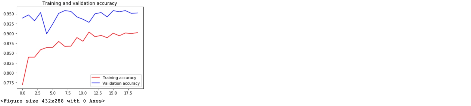
Multiclass Classifications
Rock Paper Scissors is a dataset containing 2,892 images of diverse hands in Rock/Paper/Scissors poses. (using CGI (Computer-generated images) techniques to generate).
Each image is 300×300 pixels in 24-bit color.
!wget --no-check-certificate \
    https://storage.googleapis.com/laurencemoroney-blog.appspot.com/rps.zip \
    -O /tmp/rps.zip

!wget --no-check-certificate \
    https://storage.googleapis.com/laurencemoroney-blog.appspot.com/rps-test-set.zip \
    -O /tmp/rps-test-set.zip

# -------------------

import os
import zipfile

local_zip = '/tmp/rps.zip'
zip_ref = zipfile.ZipFile(local_zip, 'r')
zip_ref.extractall('/tmp/')
zip_ref.close()

local_zip = '/tmp/rps-test-set.zip'
zip_ref = zipfile.ZipFile(local_zip, 'r')
zip_ref.extractall('/tmp/')
zip_ref.close()

# -------------------

rock_dir = os.path.join('/tmp/rps/rock')
paper_dir = os.path.join('/tmp/rps/paper')
scissors_dir = os.path.join('/tmp/rps/scissors')

print('total training rock images:', len(os.listdir(rock_dir))) # 840
print('total training paper images:', len(os.listdir(paper_dir))) # 840
print('total training scissors images:', len(os.listdir(scissors_dir))) # 840

rock_files = os.listdir(rock_dir)
print(rock_files[:10]) # ['rock04-050.png', 'rock03-067.png', 'rock04-090.png',...]

paper_files = os.listdir(paper_dir)
print(paper_files[:10]) # ['paper04-078.png', 'paper05-019.png', 'paper06-075.png',...]

scissors_files = os.listdir(scissors_dir)
print(scissors_files[:10]) # ['scissors03-005.png', 'testscissors01-057.png', 'scissors01-099.png', ...]%matplotlib inline
import matplotlib.pyplot as plt
import matplotlib.image as mpimg
nrows = 4
ncols = 4
fig = plt.gcf()
fig.set_size_inches(ncols*4, nrows*4)
pic_index = 2
next_rock = [os.path.join(rock_dir, fname)
for fname in rock_files[pic_index-2:pic_index]]
next_paper = [os.path.join(paper_dir, fname)
for fname in paper_files[pic_index-2:pic_index]]
next_scissors = [os.path.join(scissors_dir, fname)
for fname in scissors_files[pic_index-2:pic_index]]
for i, img_path in enumerate(next_rock+next_paper+next_scissors):
#print(img_path)
sp = plt.subplot(nrows, ncols, i + 1)
sp.axis('Off') # Don't show axes (or gridlines)
img = mpimg.imread(img_path)
plt.imshow(img)
plt.show()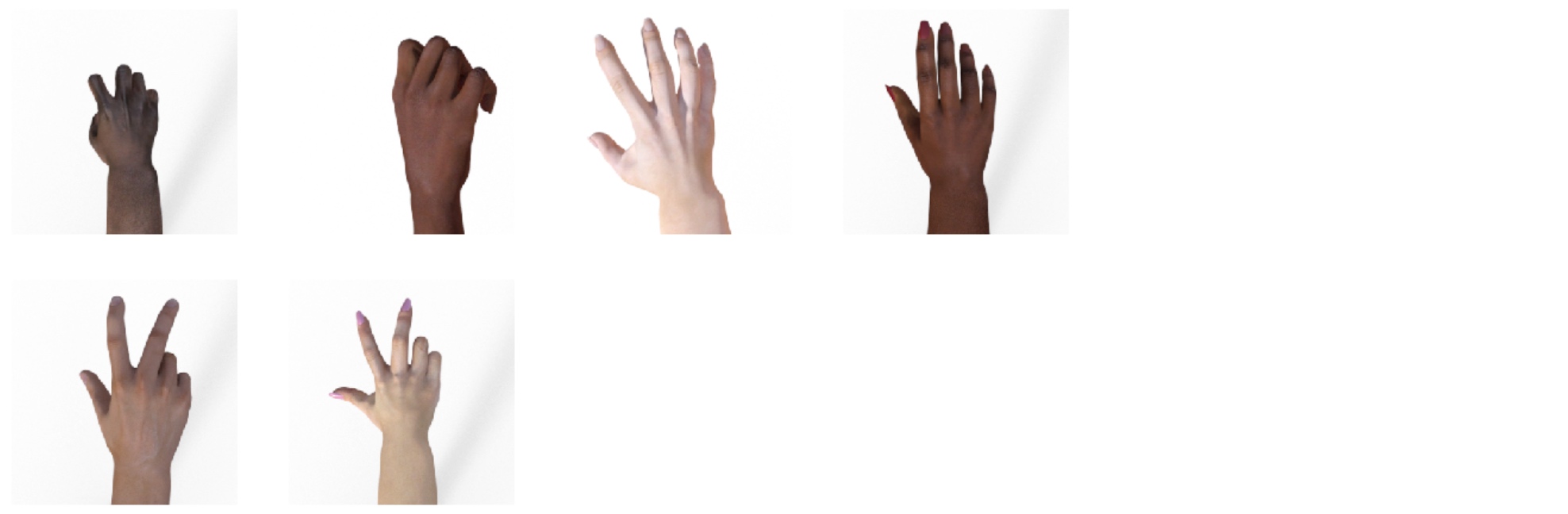
import tensorflow as tf
import keras_preprocessing
from keras_preprocessing import image
from keras_preprocessing.image import ImageDataGenerator
TRAINING_DIR = "/tmp/rps/"
training_datagen = ImageDataGenerator(
rescale = 1./255,
rotation_range=40,
width_shift_range=0.2,
height_shift_range=0.2,
shear_range=0.2,
zoom_range=0.2,
horizontal_flip=True,
fill_mode='nearest')
VALIDATION_DIR = "/tmp/rps-test-set/"
validation_datagen = ImageDataGenerator(rescale = 1./255)
train_generator = training_datagen.flow_from_directory(
TRAINING_DIR,
target_size=(150,150),
class_mode='categorical'
)
validation_generator = validation_datagen.flow_from_directory(
VALIDATION_DIR,
target_size=(150,150),
class_mode='categorical'
)
model = tf.keras.models.Sequential([
# Note the input shape is the desired size of the image 150x150 with 3 bytes color
# This is the first convolution
tf.keras.layers.Conv2D(64, (3,3), activation='relu', input_shape=(150, 150, 3)),
tf.keras.layers.MaxPooling2D(2, 2),
# The second convolution
tf.keras.layers.Conv2D(64, (3,3), activation='relu'),
tf.keras.layers.MaxPooling2D(2,2),
# The third convolution
tf.keras.layers.Conv2D(128, (3,3), activation='relu'),
tf.keras.layers.MaxPooling2D(2,2),
# The fourth convolution
tf.keras.layers.Conv2D(128, (3,3), activation='relu'),
tf.keras.layers.MaxPooling2D(2,2),
# Flatten the results to feed into a DNN
tf.keras.layers.Flatten(),
tf.keras.layers.Dropout(0.5),
# 512 neuron hidden layer
tf.keras.layers.Dense(512, activation='relu'),
tf.keras.layers.Dense(3, activation='softmax')
])
model.summary()
model.compile(loss = 'categorical_crossentropy', optimizer='rmsprop', metrics=['accuracy'])
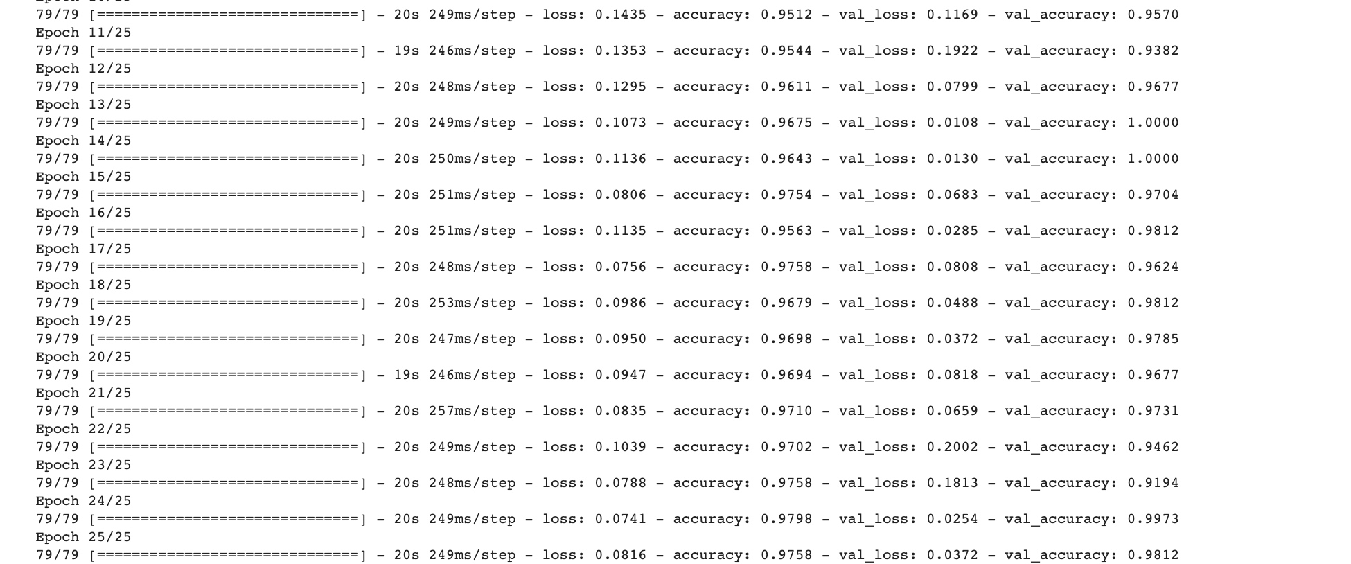
history = model.fit_generator(train_generator, epochs=25, validation_data = validation_generator, verbose = 1)
model.save("rps.h5")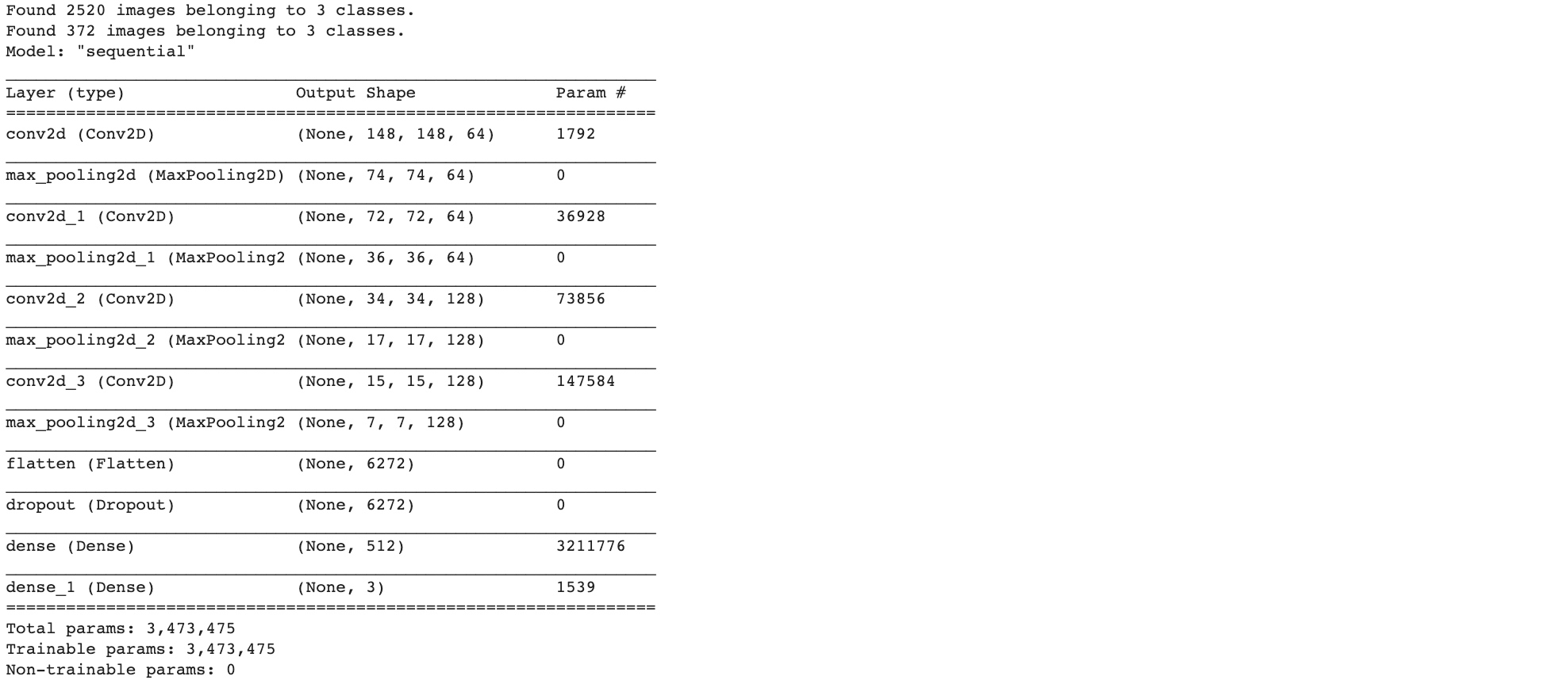
import matplotlib.pyplot as plt
acc = history.history['acc']
val_acc = history.history['val_acc']
loss = history.history['loss']
val_loss = history.history['val_loss']

epochs = range(len(acc))

plt.plot(epochs, acc, 'r', label='Training accuracy')
plt.plot(epochs, val_acc, 'b', label='Validation accuracy')
plt.title('Training and validation accuracy')
plt.legend(loc=0)
plt.figure()


plt.show()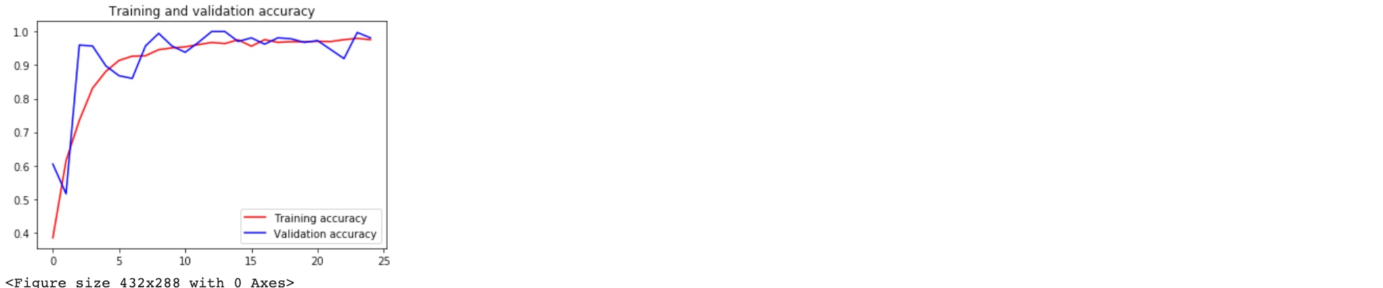
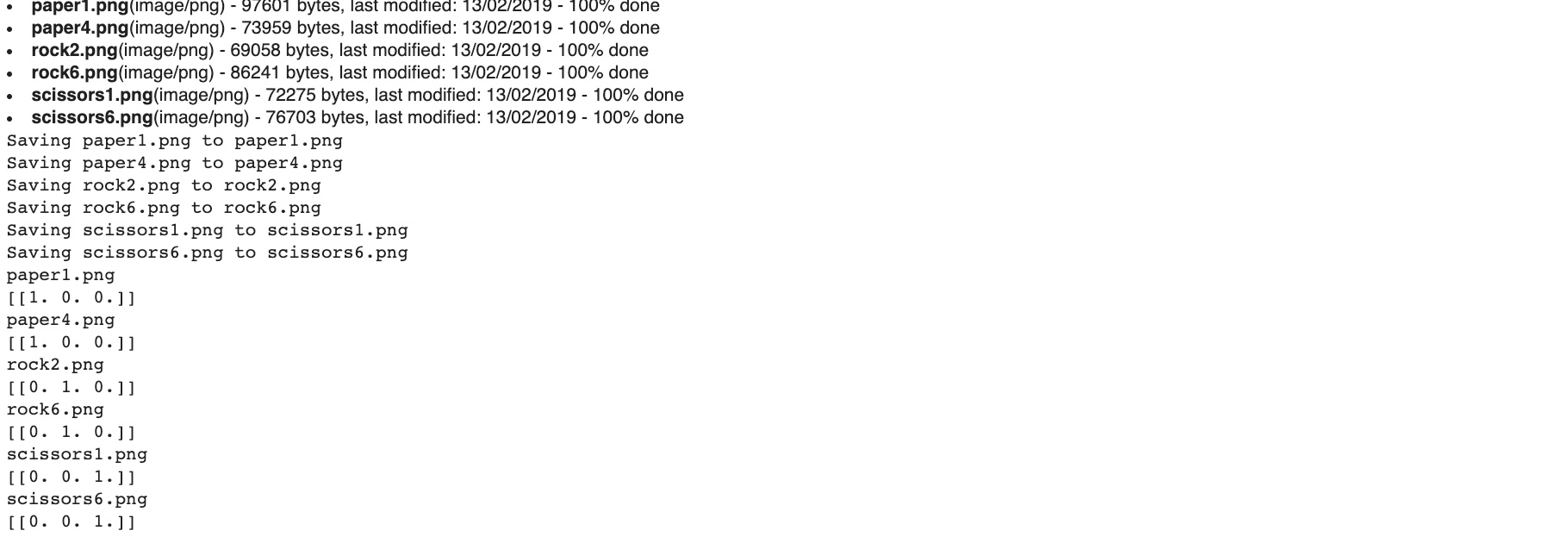
import numpy as np
from google.colab import files
from keras.preprocessing import image

uploaded = files.upload()

for fn in uploaded.keys():

  # predicting images
  path = fn
  img = image.load_img(path, target_size=(150, 150))
  x = image.img_to_array(img)
  x = np.expand_dims(x, axis=0)

  images = np.vstack([x])
  classes = model.predict(images, batch_size=10)
  print(fn)
  print(classes)
It is sorted alphabetically, so the sequence is Paper, Rock and Sicissor
Exercise: https://www.kaggle.com/datamunge/sign-language-mnist/home
import csv
import numpy as np
import tensorflow as tf
from tensorflow.keras.preprocessing.image import ImageDataGenerator
from google.colab import files

uploaded=files.upload()
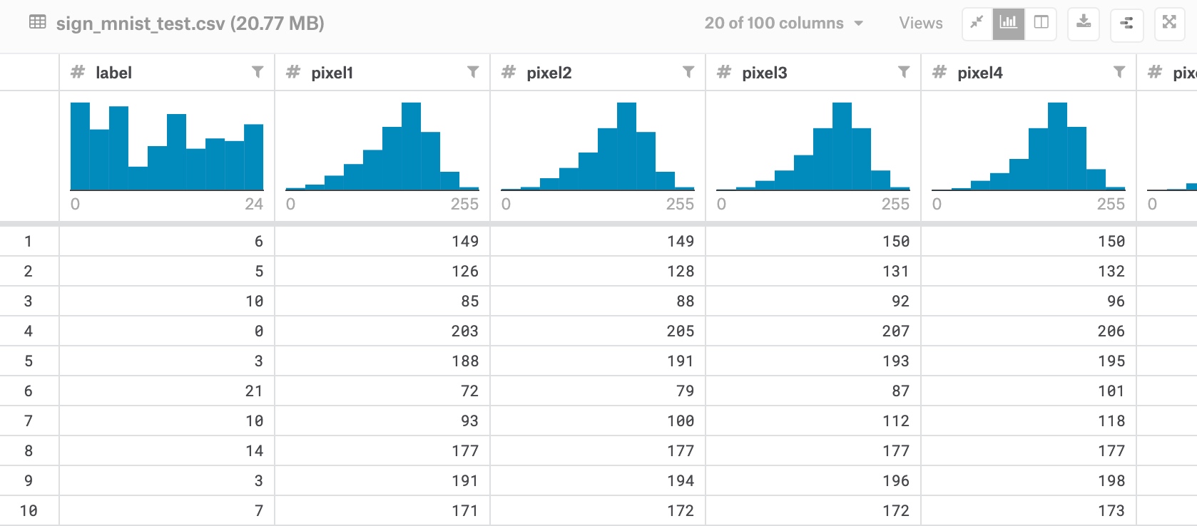 First col is label
The rest of 784 cols are pixels, need to reshape it into 28 x 28
def get_data(filename):
    with open(filename) as training_file:
        csv_reader = csv.reader(training_file, delimiter=',')
        first_line = True
        temp_images = []
        temp_labels = []
        for row in csv_reader:
            if first_line:
                # print("Ignoring first line")
                first_line = False
            else:
                temp_labels.append(row[0])
                image_data = row[1:785]
                image_data_as_array = np.array_split(image_data, 28)
                temp_images.append(image_data_as_array)
        images = np.array(temp_images).astype('float')
        labels = np.array(temp_labels).astype('float')
    return images, labels


training_images, training_labels = get_data('sign_mnist_train.csv')
testing_images, testing_labels = get_data('sign_mnist_test.csv')

print(training_images.shape)
print(training_labels.shape)
print(testing_images.shape)
print(testing_labels.shape)

# Expected output:
# (27455, 28, 28)
# (27455,)
# (7172, 28, 28)
# (7172,)
training_images = np.expand_dims(training_images, axis=3)
testing_images = np.expand_dims(testing_images, axis=3)
train_datagen = ImageDataGenerator(
rescale=1. / 255,
rotation_range=40,
width_shift_range=0.2,
height_shift_range=0.2,
shear_range=0.2,
zoom_range=0.2,
horizontal_flip=True,
fill_mode='nearest')
validation_datagen = ImageDataGenerator(
rescale=1. / 255)
print(training_images.shape)
print(testing_images.shape)
# Expected Output:
# (27455, 28, 28, 1)
# (7172, 28, 28, 1)model = tf.keras.models.Sequential([
tf.keras.layers.Conv2D(64, (3, 3), activation='relu', input_shape=(28, 28, 1)),
tf.keras.layers.MaxPooling2D(2, 2),
tf.keras.layers.Conv2D(64, (3, 3), activation='relu'),
tf.keras.layers.MaxPooling2D(2, 2),
tf.keras.layers.Flatten(),
tf.keras.layers.Dense(128, activation=tf.nn.relu),
tf.keras.layers.Dense(26, activation=tf.nn.softmax)])
model.compile(optimizer = tf.train.AdamOptimizer(),
loss = 'sparse_categorical_crossentropy',
metrics=['accuracy'])
history = model.fit_generator(train_datagen.flow(training_images, training_labels, batch_size=32),
steps_per_epoch=len(training_images) / 32,
epochs=15,
validation_data=validation_datagen.flow(testing_images, testing_labels, batch_size=32),
validation_steps=len(testing_images) / 32)
model.evaluate(testing_images, testing_labels)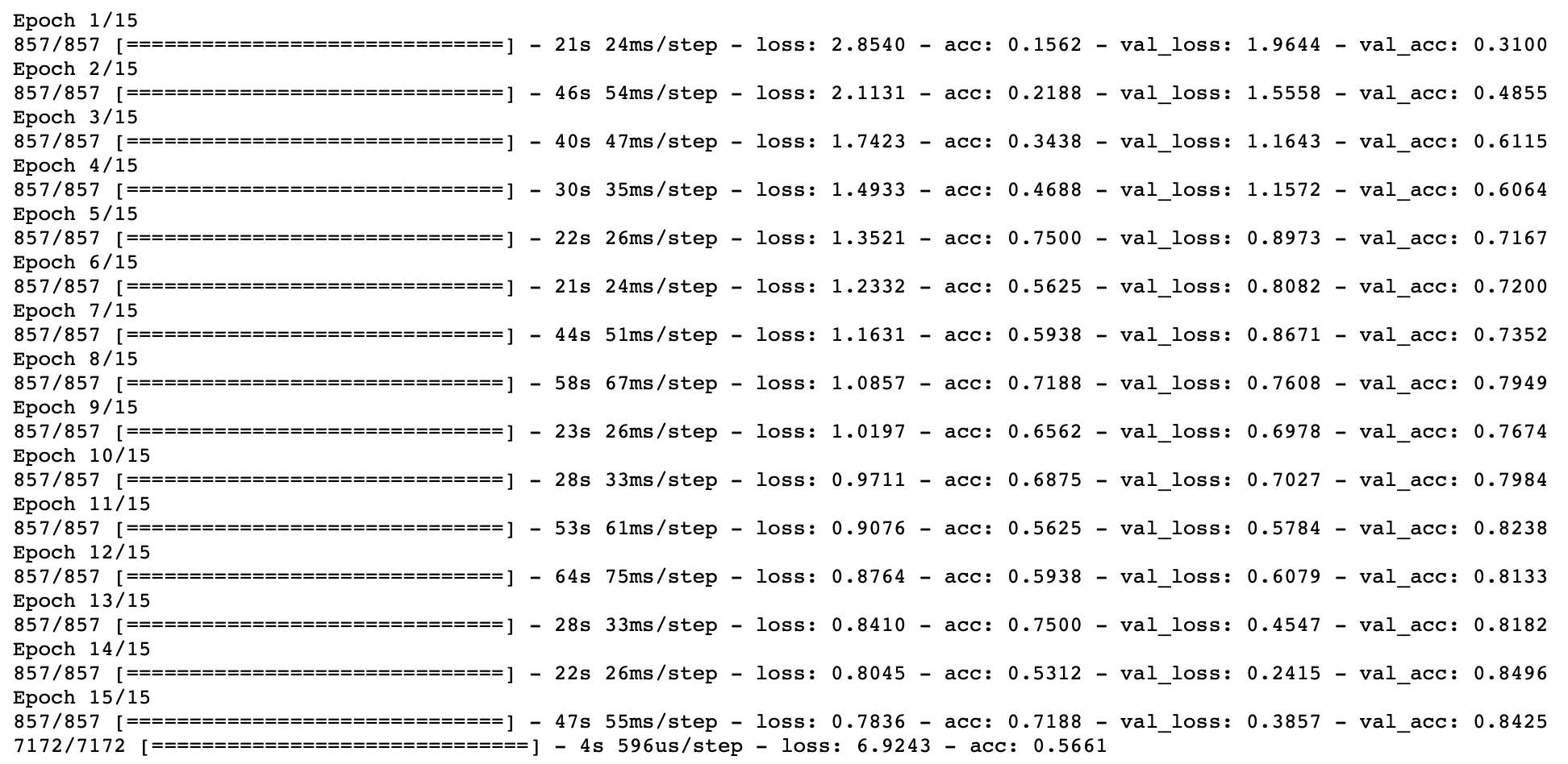
import matplotlib.pyplot as plt
acc = history.history['acc']
val_acc = history.history['val_acc']
loss = history.history['loss']
val_loss = history.history['val_loss']

epochs = range(len(acc))

plt.plot(epochs, acc, 'r', label='Training accuracy')
plt.plot(epochs, val_acc, 'b', label='Validation accuracy')
plt.title('Training and validation accuracy')
plt.legend()
plt.figure()

plt.plot(epochs, loss, 'r', label='Training Loss')
plt.plot(epochs, val_loss, 'b', label='Validation Loss')
plt.title('Training and validation loss')
plt.legend()

plt.show()