1. Introduction to TensorFlow for AI, ML, and DL
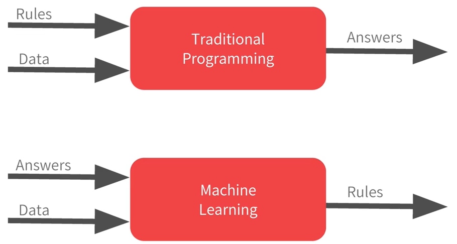
A new programming paradigm
Traditional Programming Paradigm V.S. Machine Learning Paradigm
 V.S.
V.S.
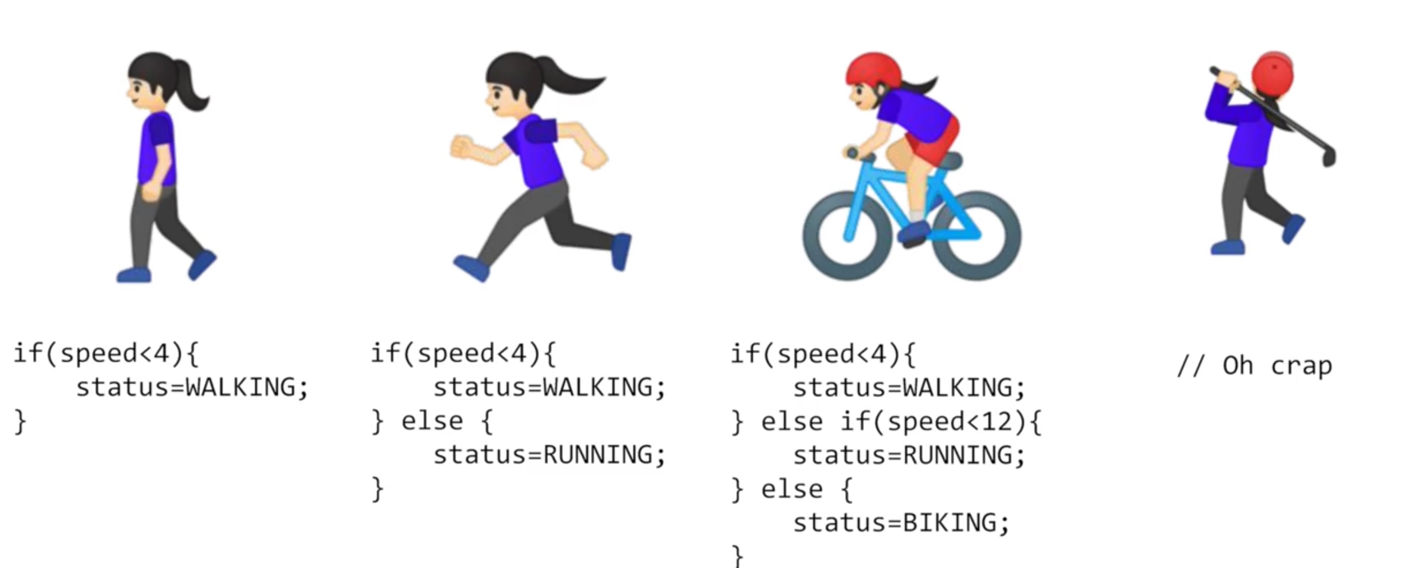
ML is all about a computer learning patterns that distinguish things
E.g.
- X = -1, 0, 1, 2, 3, 4
- Y = -3, -1, 1, 3, 5, 7
- What is the pattern between them? Answer: Y = 2X - 1
Code:
model = keras.Sequential([keras.layers.Dense(units=1, input_shape=[1])])
model.compile(optimizer='sgd', loss='mean_squared_error')

xs = np.array([-1.0, 0.0, 1.0, 2.0, 3.0, 4.0], dtype=float)
ys = np.array([-3.0, -1.0, 1.0, 3.0, 5.0, 7.0], dtype=float)

model.fit(xs, ys, epochs=500)

print(model.predict([10.0]))- Dense - define a layer of connected neurons
- compile - Make a guess, measure how good or how bad the guesses with the loss function, then use the optimizer and the data to make another guess and repeat this.
- model.fit - The process of training the neural network, where it ‘learns’ the relationship between the Xs and Ys. It will do it for the number of epochs
- model.predict - method to have it figure out the Y for a previously unknown X
- The final output is not 19 but it ended up being a little under, 2 reasons:
- train with very little data, no guarantee that for every X, the relationship will stay the same
- neural networks deal with probabilities
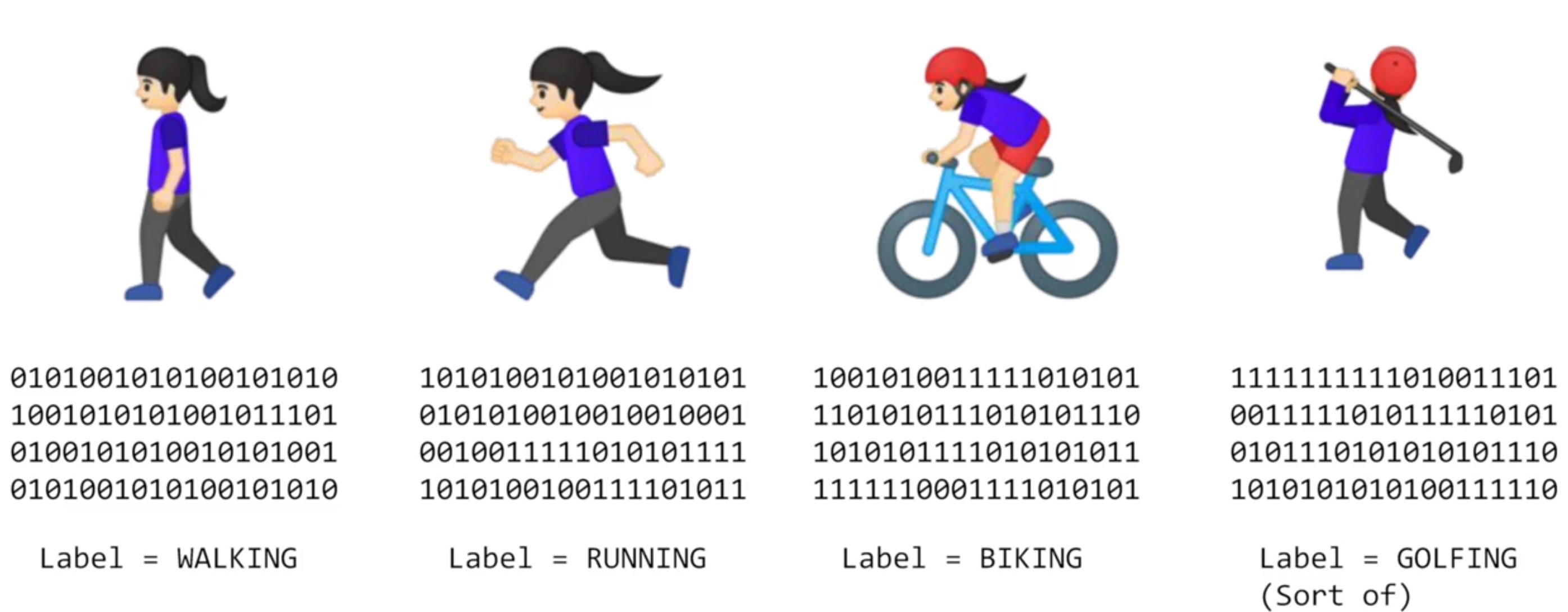
Scenarios such as Computer Vision are very difficult to solve with rules-based programming. Instead, if we feed a computer with enough data that we describe (or label) as what we want it to recognize, given that computers are really good at processing data and finding patterns that match, then we could potentially ‘train’ a system to solve a problem.
Exercise:
So, imagine if house pricing was as easy as a house costs 50k + 50k per bedroom, so that a 1 bedroom house costs 100k, a 2 bedroom house costs 150k etc.
How would you create a neural network that learns this relationship so that it would predict a 7 bedroom house as costing close to 400k etc.
Hint: Your network might work better if you scale the house price down. You don’t have to give the answer 400…it might be better to create something that predicts the number 4, and then your answer is in the ‘hundreds of thousands’ etc
import tensorflow as tf
import numpy as np
from tensorflow import keras

model = keras.Sequential([keras.layers.Dense(units=1, input_shape=[1])])
model.compile(optimizer='sgd', loss='mean_squared_error')

xs = np.array([1.0, 2.0, 3.0, 4.0, 5.0, 6.0], dtype=float)
ys = np.array([100000.0, 150000.0, 200000.0, 250000.0, 300000.0, 350000.0], dtype=float)

model.fit(xs, ys, epochs=1000)

print(model.predict([7.0])) #>>> [400596.16]
Introduction to computer vision
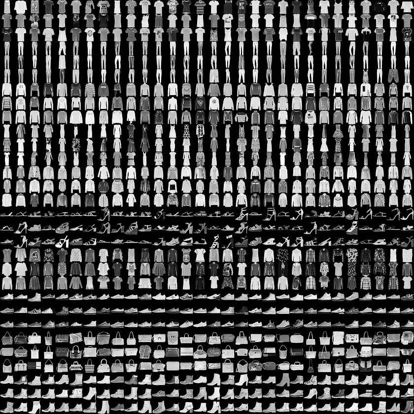
Fashion MNIST https://github.com/zalandoresearch/fashion-mnist
- 70k image
- 10 categories
- images are 28 x 28
- images are in grey scale
- can train a neural net
Code:
import tensorflow as tf
mnist = tf.keras.datasets.fashion_mnist
(training_images, training_labels), (test_images, test_labels) = mnist.load_data()
Using a number as label is to avoid bias – instead of labelling it with words in a specific language and excluding people who don’t speak that language.
import matplotlib.pyplot as plt
plt.imshow(training_images[0])
print(training_labels[0])
print(training_images[0])
Print a training image, and a training label to see.
training_images  = training_images / 255.0
test_images = test_images / 255.0
The values in the number are between 0 and 255. It’s easier if we treat all values as between 0 and 1, a process called ‘normalizing’. If normalize, the accuracy will be higher and loss will be lower
model = tf.keras.models.Sequential([tf.keras.layers.Flatten(),
                                    tf.keras.layers.Dense(128, activation=tf.nn.relu),
                                    tf.keras.layers.Dense(10, activation=tf.nn.softmax)])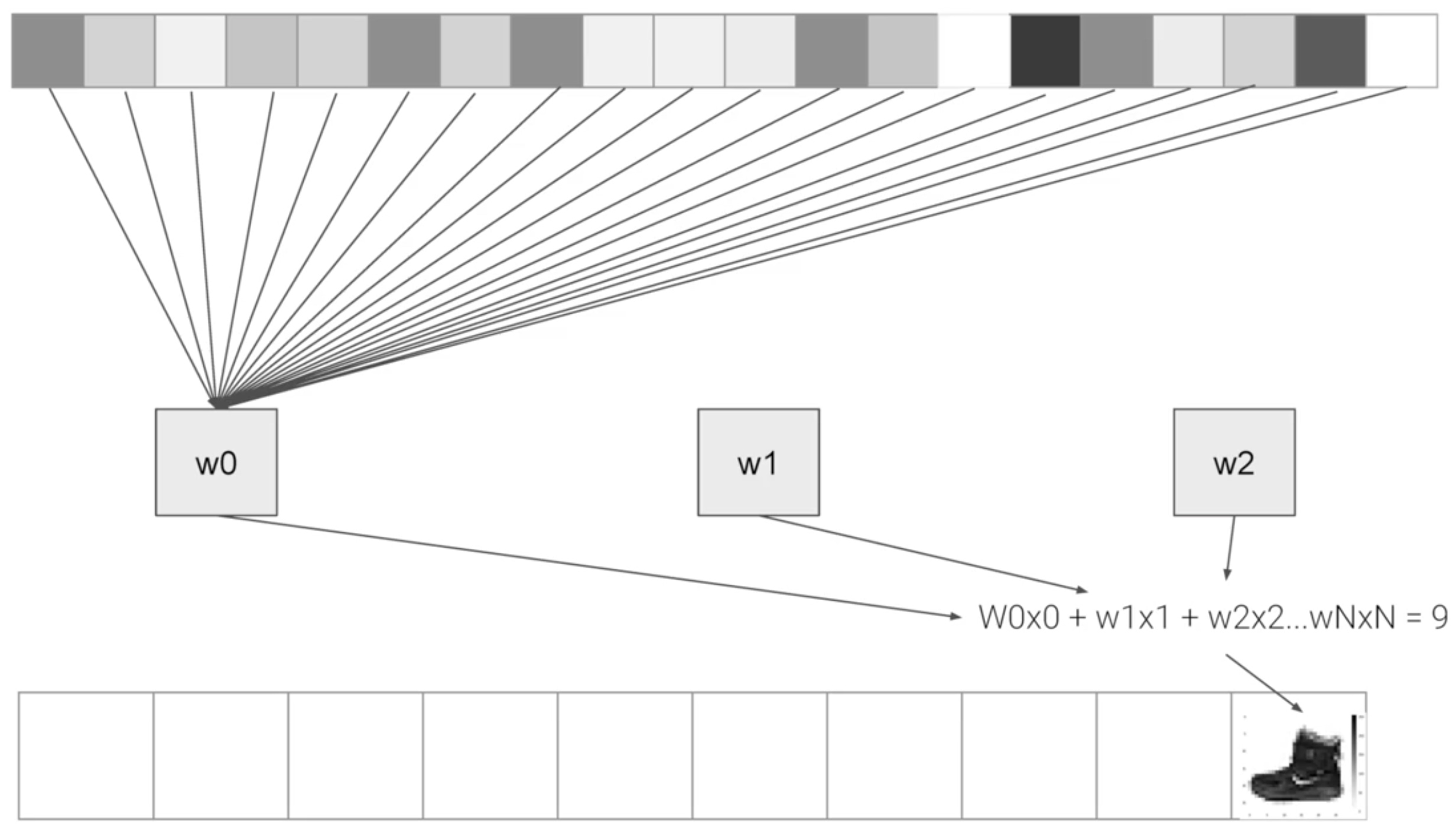
- Sequential: That defines a SEQUENCE of layers in the neural network
- Flatten: Images are square matrix. Flatten just takes that square and turns it into a 1 dimensional set.
- Dense: Adds a layer of neurons. Each layer of neurons need an activation function to tell them what to do.
- Relu effectively means “If X>0 return X, else return 0” – so it only passes values 0 or greater to the next layer in the network.
- Softmax takes a set of values, and effectively picks the biggest one, so, for example, if the output of the last layer looks like [0.1, 0.1, 0.05, 0.1, 9.5, 0.1, 0.05, 0.05, 0.05], it saves you from fishing through it looking for the biggest value, and turns it into [0,0,0,0,1,0,0,0,0]
Build model by compiling it with an optimizer and loss function and then train it 5 times.
model.compile(optimizer = tf.train.AdamOptimizer(),
              loss = 'sparse_categorical_crossentropy',
              metrics=['accuracy'])

model.fit(training_images, training_labels, epochs=5)

model.evaluate(test_images, test_labels)
Epoch 5 times, In training set, the loss is 0.2949 and accuracy is 0.8912; In test set, the loss is 0.3670 and accuracy is 0.8661
classifications = model.predict(test_images)

print(classifications[0])  # [3.6188419e-04 2.0009306e-06 1.4395033e-06 1.2049273e-07 7.3036797e-05 2.8102153e-03 2.7243374e-04 1.7680461e-02 2.1611286e-05 9.7877687e-01]
print(test_labels[0])  # 9
classifications[0] is the probability that test item[0] is each of the 10 classes. The 10th element on the list is the biggest, and the ankle boot is labelled 9
Different Scenario:
tf.keras.layers.Dense(1024, activation=tf.nn.relu)Increase to 1024 Neurons, Training takes longer, but is more accurate.- If remove the Flatten() layer, will get an error about the shape of the data. The first layer in your network should be the same shape as your data. Data is 28x28 images, and 28 layers of 28 neurons would be infeasible, so it makes more sense to ‘flatten’ that 28,28 into a 784x1.
- If final (output) layers with 5
tf.keras.layers.Dense(5, activation=tf.nn.softmax), Will get an error as soon as it finds an unexpected value. The number of neurons in the last layer should match the number of classes you are classifying for - If add another layer between the one with 512 and the final layer with 10. There isn’t a significant impact – because this is relatively simple data. For far more complex data like color images, extra layers are often necessary
- Try 15 epochs, the model probably will have a much better loss than the one with 5; Try 30 epochs, you might see the loss value stops decreasing, and sometimes increases, This is the side effect of ‘overfitting’
Set a callback function to stop iteration when you get a desired value, like 95% accuracy or less than 0.4 loss:
import tensorflow as tf
print(tf.__version__)

class myCallback(tf.keras.callbacks.Callback):
  def on_epoch_end(self, epoch, logs={}):
    if(logs.get('loss')<0.4):
      print("\nReached 60% accuracy so cancelling training!")
      self.model.stop_training = True

callbacks = myCallback()
mnist = tf.keras.datasets.fashion_mnist
(training_images, training_labels), (test_images, test_labels) = mnist.load_data()
training_images=training_images/255.0
test_images=test_images/255.0
model = tf.keras.models.Sequential([
  tf.keras.layers.Flatten(),
  tf.keras.layers.Dense(512, activation=tf.nn.relu),
  tf.keras.layers.Dense(10, activation=tf.nn.softmax)
])
model.compile(optimizer='adam', loss='sparse_categorical_crossentropy', metrics=['accuracy'])
model.fit(training_images, training_labels, epochs=5, callbacks=[callbacks])
Exercise:
Write an MNIST classifier that trains to 99% accuracy or above, and does it without a fixed number of epochs – i.e. you should stop training once you reach that level of accuracy.
Some notes:
- It should succeed in less than 10 epochs, so it is okay to change epochs to 10, but nothing larger
- When it reaches 99% or greater it should print out the string “Reached 99% accuracy so cancelling training!”
- If you add any additional variables, make sure you use the same names as the ones used in the class
import tensorflow as tf
mnist = tf.keras.datasets.mnist

(x_train, y_train),(x_test, y_test) = mnist.load_data()

x_train = x_train / 255.0
x_test = x_test / 255.0

model = tf.keras.models.Sequential([
  tf.keras.layers.Flatten(input_shape=(28, 28)),
  tf.keras.layers.Dense(512, activation=tf.nn.relu),
  tf.keras.layers.Dense(10, activation=tf.nn.softmax),
])

model.compile(optimizer='adam',
              loss='sparse_categorical_crossentropy',
              metrics=['accuracy'])

class  myCallback(tf.keras.callbacks.Callback):
  def on_epoch_end(self, epoch, logs={}):
    if(logs.get('acc')>0.99):
      print("\nReached 99% accuracy so cancelling training!")
      self.model.stop_training = True

callbacks = myCallback()

model.fit(x_train, y_train, epochs=10, callbacks=[callbacks])
Enhancing vision with convolutional neural networks
 Some convolution will change the image in such a way that the certain features in the image get emphasized:
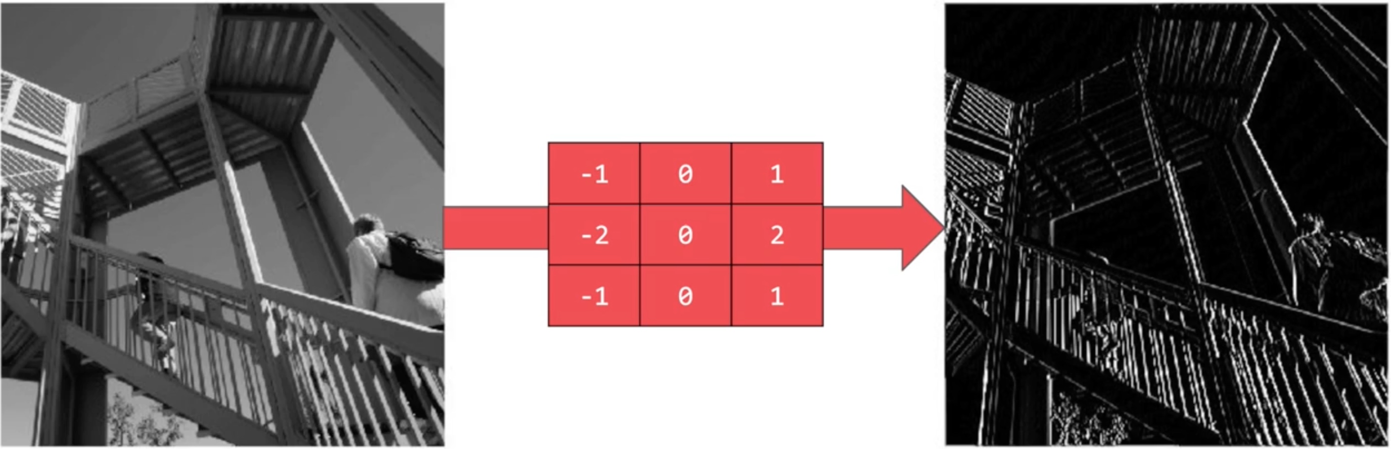 Vertical lines pop out (emphasized).
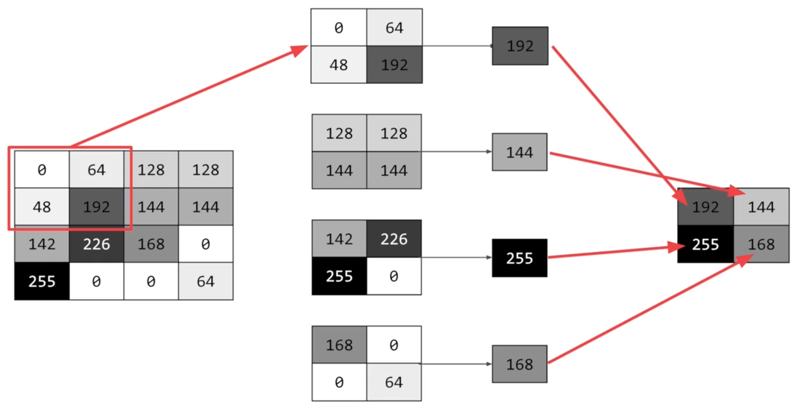
Pooling is a way of compressing an image - Max Pooling
Code:
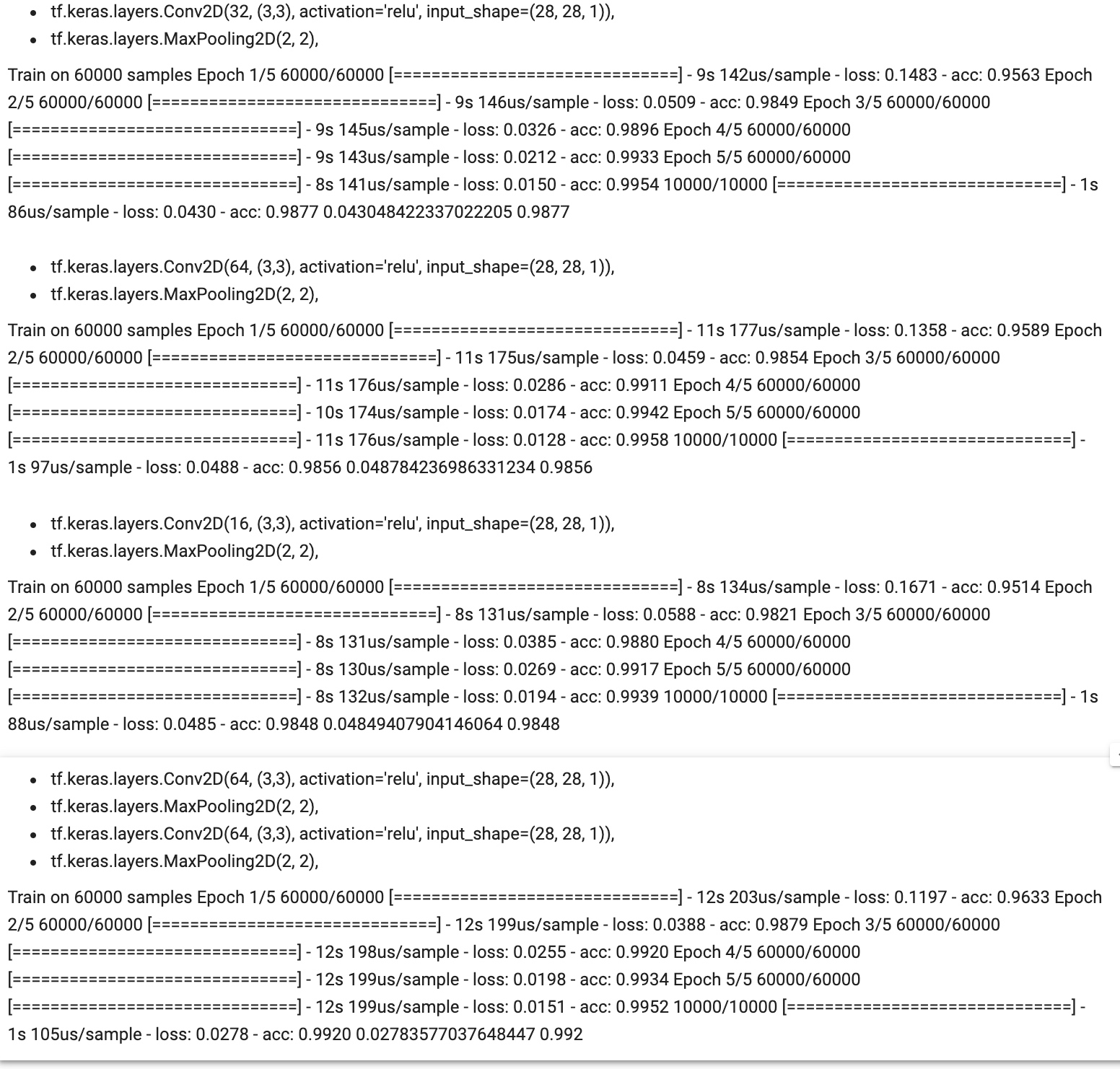
Add some layers to do convolution before the dense layers, and then the information going to the dense layers is more focussed, and possibly more accurate
import tensorflow as tf
print(tf.__version__)
mnist = tf.keras.datasets.fashion_mnist
(training_images, training_labels), (test_images, test_labels) = mnist.load_data()
training_images=training_images.reshape(60000, 28, 28, 1)
training_images=training_images / 255.0
test_images = test_images.reshape(10000, 28, 28, 1)
test_images=test_images/255.0
model = tf.keras.models.Sequential([
tf.keras.layers.Conv2D(64, (3,3), activation='relu', input_shape=(28, 28, 1)),
tf.keras.layers.MaxPooling2D(2, 2),
tf.keras.layers.Conv2D(64, (3,3), activation='relu'),
tf.keras.layers.MaxPooling2D(2,2),
tf.keras.layers.Flatten(),
tf.keras.layers.Dense(128, activation='relu'),
tf.keras.layers.Dense(10, activation='softmax')
])
model.compile(optimizer='adam', loss='sparse_categorical_crossentropy', metrics=['accuracy'])
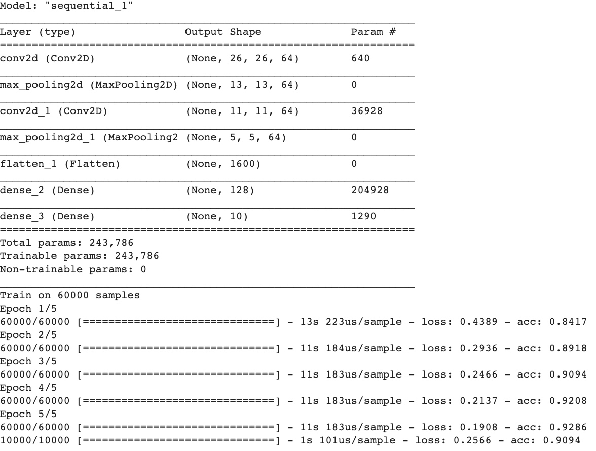
model.summary()
model.fit(training_images, training_labels, epochs=5)
test_loss = model.evaluate(test_images, test_labels)Few things to be noticed:
- Training data is reshaped to 60,000x28x28x1. Since the first convolution expects a single tensor containing everything. If you don’t do this, you’ll get an error when training as the Convolutions do not recognize the shape.
- Add a Convolution layer at the top. The parameters are:
- The number of convolutions (filter) you want to generate. Purely arbitrary, but good to start with something in the order of 32
- The size of the Convolution (filter), in this case a 3x3 grid
- The activation function to use – in this case we’ll use relu, it is equivalent of returning x when x>0, else returning 0
- In the first layer, the shape of the input data.
- Follow the Convolution with a MaxPooling layer which is designed to compress the image, while maintaining the content of the features that were highlighted by the convlution. By specifying (2,2) for the MaxPooling, the effect is to quarter the size of the image
Go with CPU
 Go with GPU (BEST)
 Go with TPU
 This code will visualize the Convolutions and Pooling, it begins to see common features between them emerge:
import matplotlib.pyplot as plt
f, axarr = plt.subplots(3,4)
# Below 3 images both are shoes
FIRST_IMAGE=0
SECOND_IMAGE=23
THIRD_IMAGE=28
CONVOLUTION_NUMBER = 1
from tensorflow.keras import models
layer_outputs = [layer.output for layer in model.layers]
print(layer_outputs)  # All Layer Tensors
print(model.input)  # Input Tensor
activation_model = tf.keras.models.Model(inputs = model.input, outputs = layer_outputs)
for x in range(0,4):  # First fourth layers: CONV2D , MAXPOOLING, CONV2D , MAXPOOLING
  f1 = activation_model.predict(test_images[FIRST_IMAGE].reshape(1, 28, 28, 1))[x]
  axarr[0,x].imshow(f1[0, : , :, CONVOLUTION_NUMBER], cmap='inferno')
  axarr[0,x].grid(False)
  f2 = activation_model.predict(test_images[SECOND_IMAGE].reshape(1, 28, 28, 1))[x]
  axarr[1,x].imshow(f2[0, : , :, CONVOLUTION_NUMBER], cmap='inferno')
  axarr[1,x].grid(False)
  f3 = activation_model.predict(test_images[THIRD_IMAGE].reshape(1, 28, 28, 1))[x]
  axarr[2,x].imshow(f3[0, : , :, CONVOLUTION_NUMBER], cmap='inferno')
  axarr[2,x].grid(False)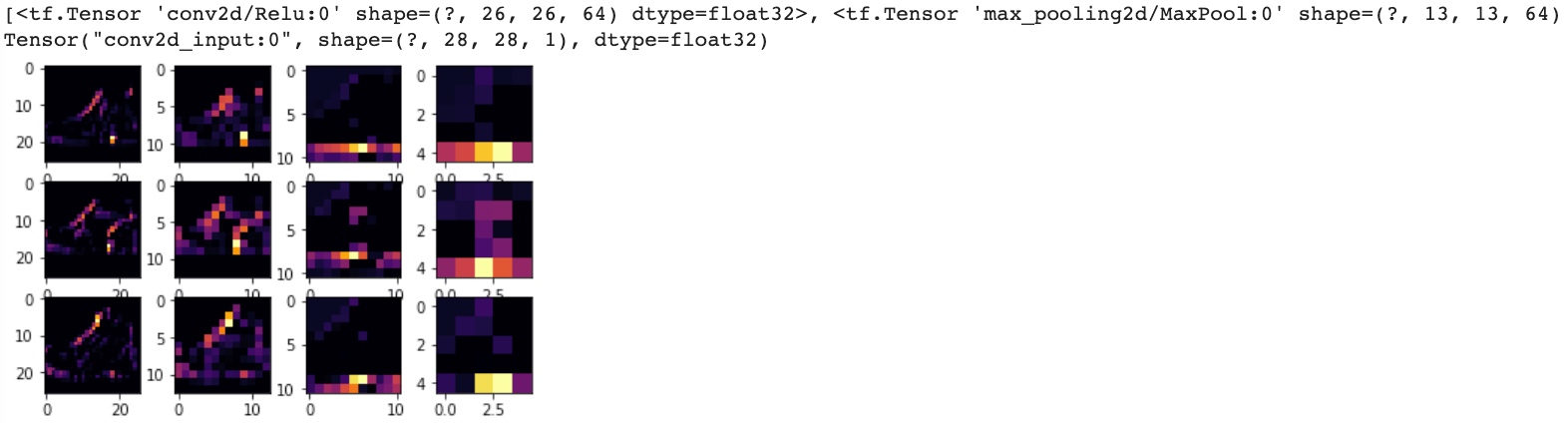
Explore how convolutions work by creating a basic convolution on a 2D Grey Scale image - https://lodev.org/cgtutor/filtering.html#Convolution:
import cv2
import numpy as np
from scipy import misc
import matplotlib.pyplot as plt

i = misc.ascent() # load the image by taking the 'ascent' image from scipy

plt.grid(False)
plt.gray()
plt.axis('off')
plt.imshow(i)
plt.show()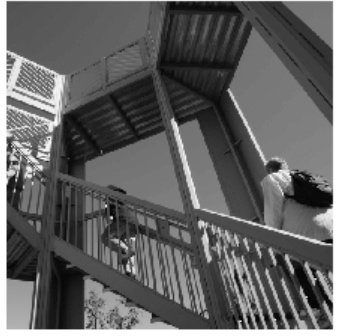
Create a filter as a 3x3 array:
# This filter detects edges nicely
# It creates a convolution that only passes through sharp edges and straight lines.
#filter = [ [0, 1, 0], [1, -4, 1], [0, 1, 0]]
filter = [ [-1, -2, -1], [0, 0, 0], [1, 2, 1]]
#filter = [ [-1, 0, 1], [-2, 0, 2], [-1, 0, 1]]
# If all the digits in the filter don't add up to 0 or 1, you should probably do a weight to get it to do so.
# For example, if your weights are 1,1,1 1,2,1 1,1,1
# They add up to 10, so you would set a weight of .1 if you want to normalize them
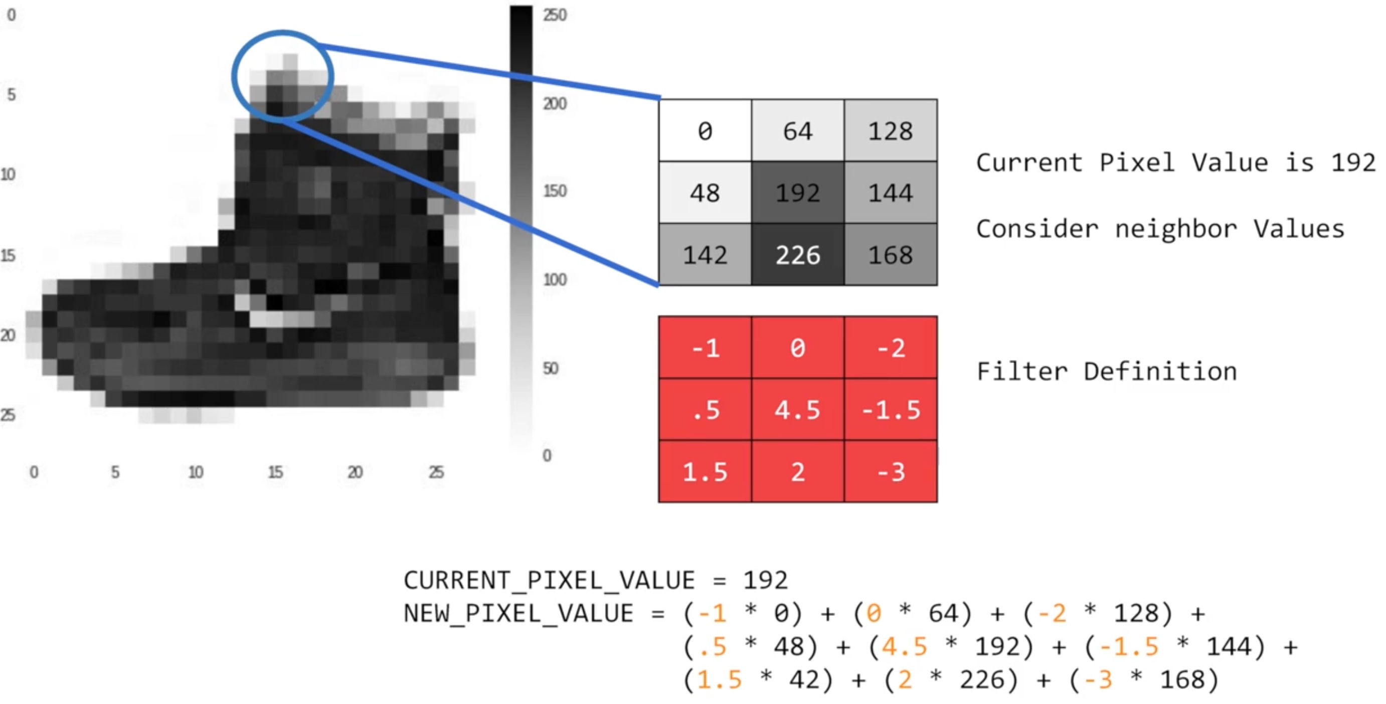
weight = 1Create a convolution by iterating over the image, leaving a 1 pixel margin, and multiply out each of the neighbors of the current pixel by the value defined in the filter.
i_transformed = np.copy(i)
size_x = i_transformed.shape[0]
size_y = i_transformed.shape[1]
print(size_x,size_y)  # 512,512

for x in range(1,size_x-1):
  for y in range(1,size_y-1):
      convolution = 0.0
      convolution = convolution + (i[x - 1, y-1] * filter[0][0])
      convolution = convolution + (i[x, y-1] * filter[0][1])
      convolution = convolution + (i[x + 1, y-1] * filter[0][2])
      convolution = convolution + (i[x-1, y] * filter[1][0])
      convolution = convolution + (i[x, y] * filter[1][1])
      convolution = convolution + (i[x+1, y] * filter[1][2])
      convolution = convolution + (i[x-1, y+1] * filter[2][0])
      convolution = convolution + (i[x, y+1] * filter[2][1])
      convolution = convolution + (i[x+1, y+1] * filter[2][2])
      convolution = convolution * weight
      if(convolution<0):
        convolution=0
      if(convolution>255):
        convolution=255
      i_transformed[x, y] = convolution


# Plot the image. Note the size of the axes -- they are 512 by 512
print(i_transformed.shape) # 512,512
plt.gray()
plt.grid(False)
plt.imshow(i_transformed)
#plt.axis('off')
plt.show() 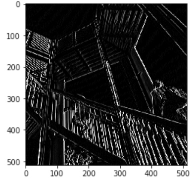
(2, 2) max pooling, the new image will be 1⁄4 the size of the old:
new_x = int(size_x/2)
new_y = int(size_y/2)
newImage = np.zeros((new_x, new_y))
for x in range(0, size_x, 2):
  for y in range(0, size_y, 2):
    pixels = []
    pixels.append(i_transformed[x, y])
    pixels.append(i_transformed[x+1, y])
    pixels.append(i_transformed[x, y+1])
    pixels.append(i_transformed[x+1, y+1])
    newImage[int(x/2),int(y/2)] = max(pixels)

# Plot the image. Note the size of the axes -- now 256 pixels instead of 512
plt.gray()
plt.grid(False)
plt.imshow(newImage)
#plt.axis('off')
plt.show() 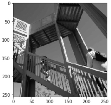
Exercise:
For your exercise see if you can improve MNIST to 99.8% accuracy or more using only a single convolutional layer and a single MaxPooling 2D. You should stop training once the accuracy goes above this amount. It should happen in less than 20 epochs, so it’s ok to hard code the number of epochs for training, but your training must end once it hits the above metric. If it doesn’t, then you’ll need to redesign your layers.
import tensorflow as tf
print(tf.__version__)

class myCallback(tf.keras.callbacks.Callback):
  def on_epoch_end(self, epoch, logs={}):
    if(logs.get('acc')>0.998):
      print("\nReached 99.8% accuracy so cancelling training!")
      self.model.stop_training = True

callbacks = myCallback()


mnist = tf.keras.datasets.mnist  ## not fashion mnist
(training_images, training_labels), (test_images, test_labels) = mnist.load_data()
training_images=training_images.reshape(60000, 28, 28, 1)
training_images=training_images / 255.0
test_images = test_images.reshape(10000, 28, 28, 1)
test_images=test_images/255.0
model = tf.keras.models.Sequential([
  tf.keras.layers.Conv2D(32, (3,3), activation='relu', input_shape=(28, 28, 1)),
  tf.keras.layers.MaxPooling2D(2, 2),
  tf.keras.layers.Flatten(),
  tf.keras.layers.Dense(128, activation='relu'),
  tf.keras.layers.Dense(10, activation='softmax')
])
model.compile(optimizer='adam', loss='sparse_categorical_crossentropy', metrics=['accuracy'])
model.fit(training_images, training_labels, epochs=13, callbacks=[callbacks])
test_loss, test_acc = model.evaluate(test_images, test_labels)
print(test_loss, test_acc)
Different Scenario of MNIST Dataset:
Using real world images
Image generator in Tensorflow - it can flow images from a directory and perform operations such as resizing them on the fly
Neural network to classify Horses or Humans:
Load the data:
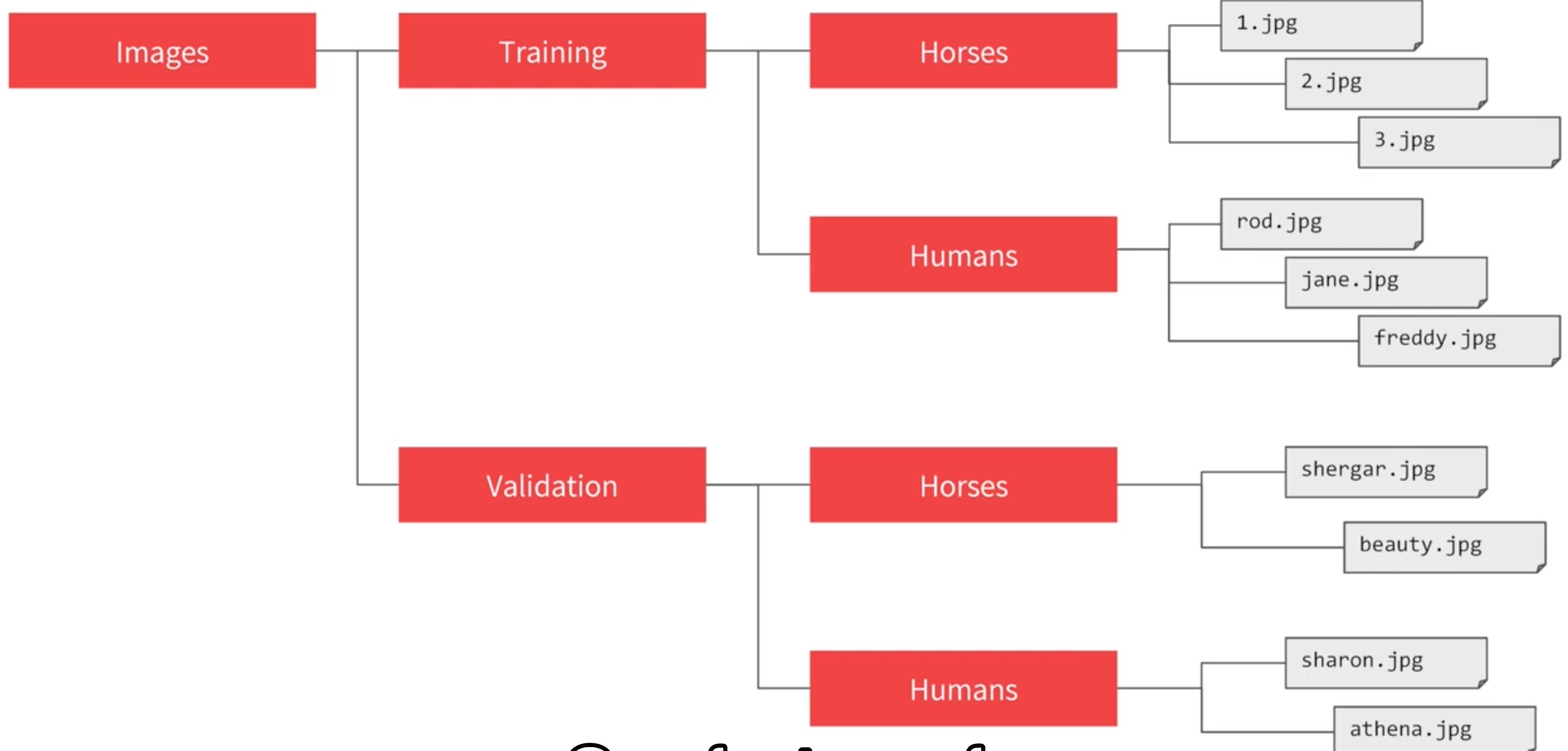
The dataset does not explicitly label the images as horses or humans. ImageGenerator is used to read images from subdirectories, and automatically label them from the name of that subdirectory.
!wget --no-check-certificate https://storage.googleapis.com/laurencemoroney-blog.appspot.com/horse-or-human.zip -O /tmp/horse-or-human.zip

!wget --no-check-certificate https://storage.googleapis.com/laurencemoroney-blog.appspot.com/validation-horse-or-human.zip -O /tmp/validation-horse-or-human.zip

import os
import zipfile

local_zip = '/tmp/horse-or-human.zip'
zip_ref = zipfile.ZipFile(local_zip, 'r')
zip_ref.extractall('/tmp/horse-or-human')
local_zip = '/tmp/validation-horse-or-human.zip'
zip_ref = zipfile.ZipFile(local_zip, 'r')
zip_ref.extractall('/tmp/validation-horse-or-human')
zip_ref.close()

# Directory with our training horse pictures
train_horse_dir = os.path.join('/tmp/horse-or-human/horses')
# Directory with our training human pictures
train_human_dir = os.path.join('/tmp/horse-or-human/humans')
# Directory with our validation horse pictures
validation_horse_dir = os.path.join('/tmp/validation-horse-or-human/horses')
# Directory with our validation human pictures
validation_human_dir = os.path.join('/tmp/validation-horse-or-human/humans')

train_horse_names = os.listdir(train_horse_dir)
print(train_horse_names[:10])  # ['horse07-8.png', 'horse44-6.png', 'horse03-7.png', 'horse22-5.png'...]
train_human_names = os.listdir(train_human_dir)
print(train_human_names[:10])  # ['human05-05.png', 'human11-18.png', 'human17-25.png', 'human06-14.png'....]
validation_horse_hames = os.listdir(validation_horse_dir)
print(validation_horse_hames[:10])
validation_human_names = os.listdir(validation_human_dir)
print(validation_human_names[:10])

print('total training horse images:', len(os.listdir(train_horse_dir)))  # 500
print('total training human images:', len(os.listdir(train_human_dir)))  # 527
print('total validation horse images:', len(os.listdir(validation_horse_dir))) # 128
print('total validation human images:', len(os.listdir(validation_human_dir))) # 128
Visualize the data:
%matplotlib inline
import matplotlib.pyplot as plt
import matplotlib.image as mpimg
# Parameters for our graph; we'll output images in a 4x4 configuration
nrows = 4
ncols = 4
# Index for iterating over images
pic_index = 0
# Set up matplotlib fig, and size it to fit 4x4 pics
fig = plt.gcf()
fig.set_size_inches(ncols * 4, nrows * 4)
pic_index += 8
next_horse_pix = [os.path.join(train_horse_dir, fname)
for fname in train_horse_names[pic_index-8:pic_index]]
next_human_pix = [os.path.join(train_human_dir, fname)
for fname in train_human_names[pic_index-8:pic_index]]
for i, img_path in enumerate(next_horse_pix+next_human_pix):
# Set up subplot; subplot indices start at 1
sp = plt.subplot(nrows, ncols, i + 1)
sp.axis('Off') # Don't show axes (or gridlines)
img = mpimg.imread(img_path)
plt.imshow(img)
plt.show()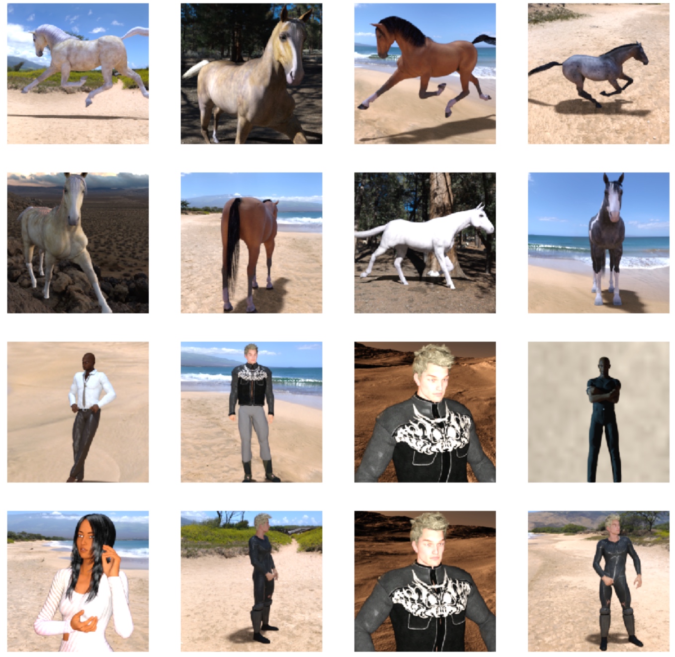 build model:
import tensorflow as tf
model = tf.keras.models.Sequential([
# Note the input shape is the desired size of the image 300x300 with 3 bytes color
# This is the first convolution
tf.keras.layers.Conv2D(16, (3,3), activation='relu', input_shape=(300, 300, 3)),
tf.keras.layers.MaxPooling2D(2, 2),
# The second convolution
tf.keras.layers.Conv2D(32, (3,3), activation='relu'),
tf.keras.layers.MaxPooling2D(2,2),
# The third convolution
tf.keras.layers.Conv2D(64, (3,3), activation='relu'),
tf.keras.layers.MaxPooling2D(2,2),
# The fourth convolution
tf.keras.layers.Conv2D(64, (3,3), activation='relu'),
tf.keras.layers.MaxPooling2D(2,2),
# The fifth convolution
tf.keras.layers.Conv2D(64, (3,3), activation='relu'),
tf.keras.layers.MaxPooling2D(2,2),
# Flatten the results to feed into a DNN
tf.keras.layers.Flatten(),
# 512 neuron hidden layer
tf.keras.layers.Dense(512, activation='relu'),
# Only 1 output neuron. It will contain a value from 0-1 where 0 for 1 class ('horses') and 1 for the other ('humans')
tf.keras.layers.Dense(1, activation='sigmoid') # end network with a sigmoid activation, because it is a two-class classification problem
])
model.summary()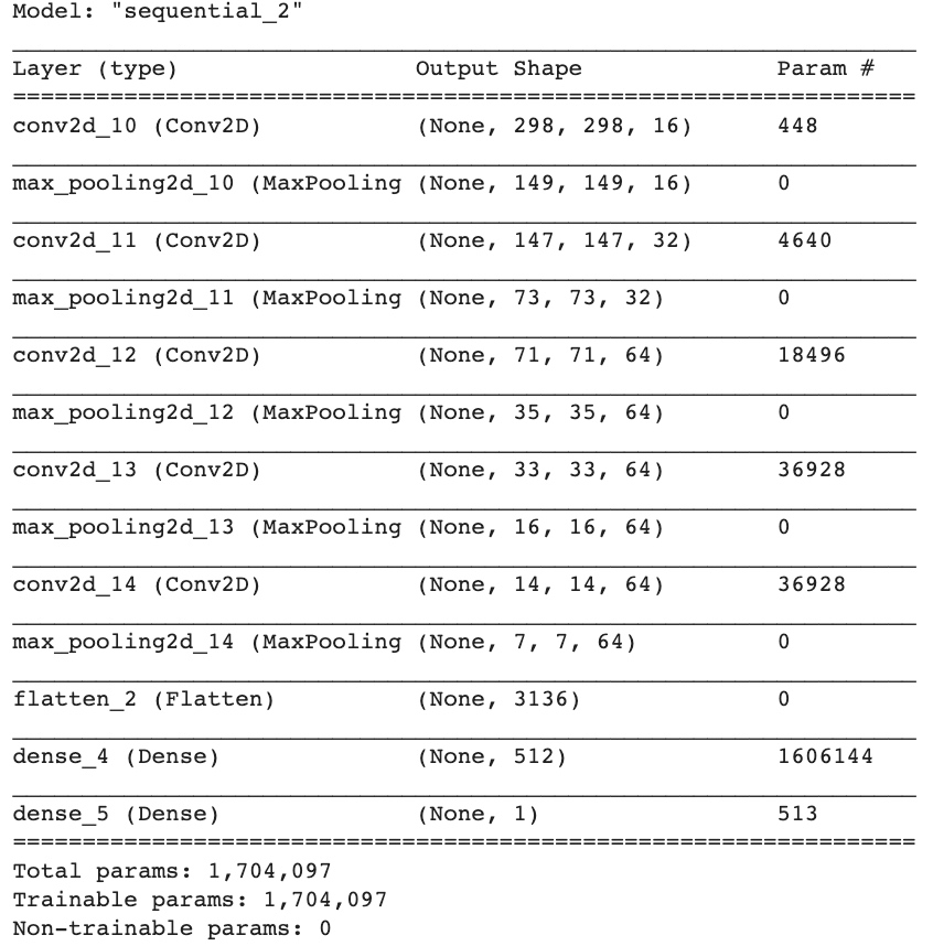 The ‘output shape’ column shows how the size of your feature map evolves in each successive layer. The convolution layers reduce the size of the feature maps by a bit due to padding, and each pooling layer halves the dimensions.
Configure the specifications for model training:
from tensorflow.keras.optimizers import RMSprop

model.compile(loss='binary_crossentropy',
              optimizer=RMSprop(lr=0.001),
              metrics=['acc'])
When defined the model, a new loss function called ‘Binary Crossentropy’, and a new optimizer called ‘RMSProp’ are leveraged.
Data Preprocessing:
- Data generators will read pictures in source folders, convert them to float32 tensors, and feed them (with their labels) to network.
- Generators will yield batches of images of size 300x300 and their labels (binary).
- Can use
rescaleparameter to normalize the data - Can instantiate generators of augmented image batches (and their labels) via
.flow(data, labels)or.flow_from_directory(directory) These generators can then be used with the Keras model methods that accept data generators as inputs:
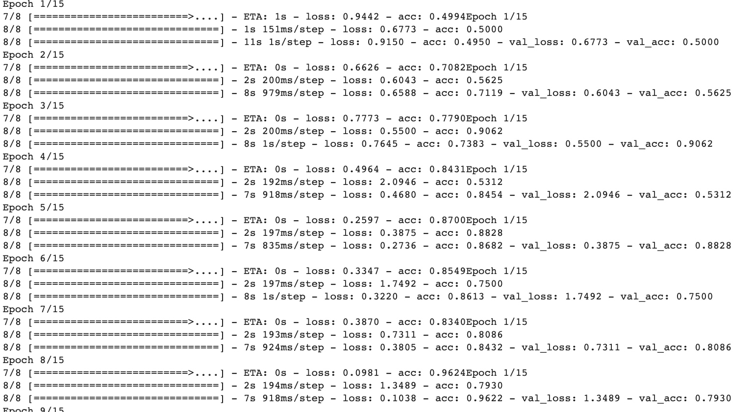
fit_generator,evaluate_generator, andpredict_generator.from tensorflow.keras.preprocessing.image import ImageDataGenerator # All images will be rescaled by 1./255 train_datagen = ImageDataGenerator(rescale=1/255) validation_datagen = ImageDataGenerator(rescale=1/255) # Flow training images in batches of 128 using train_datagen generator train_generator = train_datagen.flow_from_directory( '/tmp/horse-or-human/', # This is the source directory for training images target_size=(300, 300), # All images will be resized to 150x150 batch_size=128, # Since we use binary_crossentropy loss, we need binary labels class_mode='binary') # Flow training images in batches of 128 using train_datagen generator validation_generator = validation_datagen.flow_from_directory( '/tmp/validation-horse-or-human/', # This is the source directory for training images target_size=(300, 300), # All images will be resized to 150x150 batch_size=32, # Since we use binary_crossentropy loss, we need binary labels class_mode='binary') history = model.fit_generator( train_generator, steps_per_epoch=8, epochs=15, verbose=1, # it decides how detail the training process display validation_data = validation_generator, validation_steps=8)
Run the model:
import numpy as np
from google.colab import files  # colab code
from keras.preprocessing import image

uploaded = files.upload() # colab code

for fn in uploaded.keys(): # colab code

  # predicting images
  path = '/content/' + fn
  img = image.load_img(path, target_size=(300, 300))
  x = image.img_to_array(img)
  x = np.expand_dims(x, axis=0)

  images = np.vstack([x])
  classes = model.predict(images, batch_size=10)
  print(classes[0])
  if classes[0]>0.5:
    print(fn + " is a human")
  else:
    print(fn + " is a horse")
Visualize how an input gets transformed as it goes through the convnet:
import numpy as np
import random
from tensorflow.keras.preprocessing.image import img_to_array, load_img
# Let's define a new Model that will take an image as input, and will output
# intermediate representations for all layers in the previous model after the first.
successive_outputs = [layer.output for layer in model.layers[1:]]
#visualization_model = Model(img_input, successive_outputs)
visualization_model = tf.keras.models.Model(inputs = model.input, outputs = successive_outputs)
# Let's prepare a random input image from the training set.
horse_img_files = [os.path.join(train_horse_dir, f) for f in train_horse_names]
human_img_files = [os.path.join(train_human_dir, f) for f in train_human_names]
img_path = random.choice(horse_img_files + human_img_files)
img = load_img(img_path, target_size=(300, 300)) # this is a PIL image
x = img_to_array(img) # Numpy array with shape (150, 150, 3)
x = x.reshape((1,) + x.shape) # Numpy array with shape (1, 150, 150, 3)
# Rescale by 1/255
x /= 255
# Let's run our image through our network, thus obtaining all intermediate representations for this image.
successive_feature_maps = visualization_model.predict(x)
# These are the names of the layers, so can have them as part of our plot
layer_names = [layer.name for layer in model.layers]
# Now let's display our representations
for layer_name, feature_map in zip(layer_names, successive_feature_maps):
if len(feature_map.shape) == 4:
# Just do this for the conv / maxpool layers, not the fully-connected layers
n_features = feature_map.shape[-1] # number of features in feature map
# The feature map has shape (1, size, size, n_features)
size = feature_map.shape[1]
# We will tile our images in this matrix
display_grid = np.zeros((size, size * n_features))
for i in range(n_features):
# Postprocess the feature to make it visually palatable
x = feature_map[0, :, :, i]
x -= x.mean()
x /= x.std()
x *= 64
x += 128
x = np.clip(x, 0, 255).astype('uint8')
# We'll tile each filter into this big horizontal grid
display_grid[:, i * size : (i + 1) * size] = x
# Display the grid
scale = 20. / n_features
plt.figure(figsize=(scale * n_features, scale))
plt.title(layer_name)
plt.grid(False)
plt.imshow(display_grid, aspect='auto', cmap='viridis')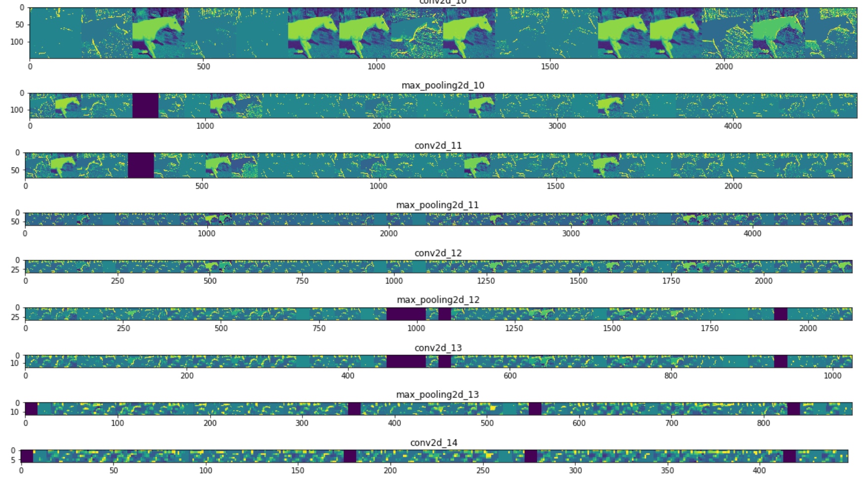 It goes from the raw pixels of the images to increasingly abstract and compact representations. The representations downstream start highlighting what the network pays attention to, and they show fewer and fewer features being ‘activated’; most are set to zero. This is called ‘sparsity’.
Clean up - terminate the kernel and free memory resources:
import os, signal
os.kill(os.getpid(), signal.SIGKILL)
Exercise:
Below is code with a link to a happy or sad dataset which contains 80 images, 40 happy and 40 sad. Create a convolutional neural network that trains to 100% accuracy on these images, which cancels training upon hitting training accuracy of >.999
Hint – it will work best with 3 convolutional layers.
import tensorflow as tf
import os
import zipfile

DESIRED_ACCURACY = 0.999

!wget --no-check-certificate \
    "https://storage.googleapis.com/laurencemoroney-blog.appspot.com/happy-or-sad.zip" \
    -O "/tmp/happy-or-sad.zip"

zip_ref = zipfile.ZipFile("/tmp/happy-or-sad.zip", 'r')
zip_ref.extractall("/tmp/h-or-s")
zip_ref.close()

class myCallback(tf.keras.callbacks.Callback):
  def on_epoch_end(self, epoch, logs={}):
    if(logs.get('acc')>DESIRED_ACCURACY):
      print("\nReached 99.9% accuracy so cancelling training!")
      self.model.stop_training = True

callbacks = myCallback()

model = tf.keras.models.Sequential([
    tf.keras.layers.Conv2D(16, (3,3), activation='relu', input_shape=(150, 150, 3)),
    tf.keras.layers.MaxPooling2D(2, 2),
    tf.keras.layers.Conv2D(32, (3,3), activation='relu'),
    tf.keras.layers.MaxPooling2D(2,2),
    tf.keras.layers.Conv2D(32, (3,3), activation='relu'),
    tf.keras.layers.MaxPooling2D(2,2),
    tf.keras.layers.Flatten(),
    tf.keras.layers.Dense(512, activation='relu'),
    tf.keras.layers.Dense(1, activation='sigmoid')
])

from tensorflow.keras.optimizers import RMSprop

model.compile(loss='binary_crossentropy',
              optimizer=RMSprop(lr=0.001),
              metrics=['acc'])

from tensorflow.keras.preprocessing.image import ImageDataGenerator

train_datagen = ImageDataGenerator(rescale=1/255)

train_generator = train_datagen.flow_from_directory(
        "/tmp/h-or-s",
        target_size=(150, 150),
        batch_size=10,
        class_mode='binary')

# Expected output: 'Found 80 images belonging to 2 classes'

history = model.fit_generator(
      train_generator,
      steps_per_epoch=2,
      epochs=15,
      verbose=1,
      callbacks=[callbacks])